Introduction
The issue of searching through many different potential solutions can often come up in computer science. When problems get more complex, this can take a lot of time and memory. Algorithms such as backtracking and branch-and-bound techniques can be used to search for solutions whilst avoiding unnecessary searches. They can be used to identify any potential solutions that will not create a valid or optimum solution.
Backtracking focuses on discarding partial solutions that do not satisfy the constraints of the problem, whereas branch and bound uses calculated bounds to discard any options that would not improve the current most optimum solution. This can help developers solve more complex problems in an efficient way.
What are Backtracking and Branch and Bound Algorithms?
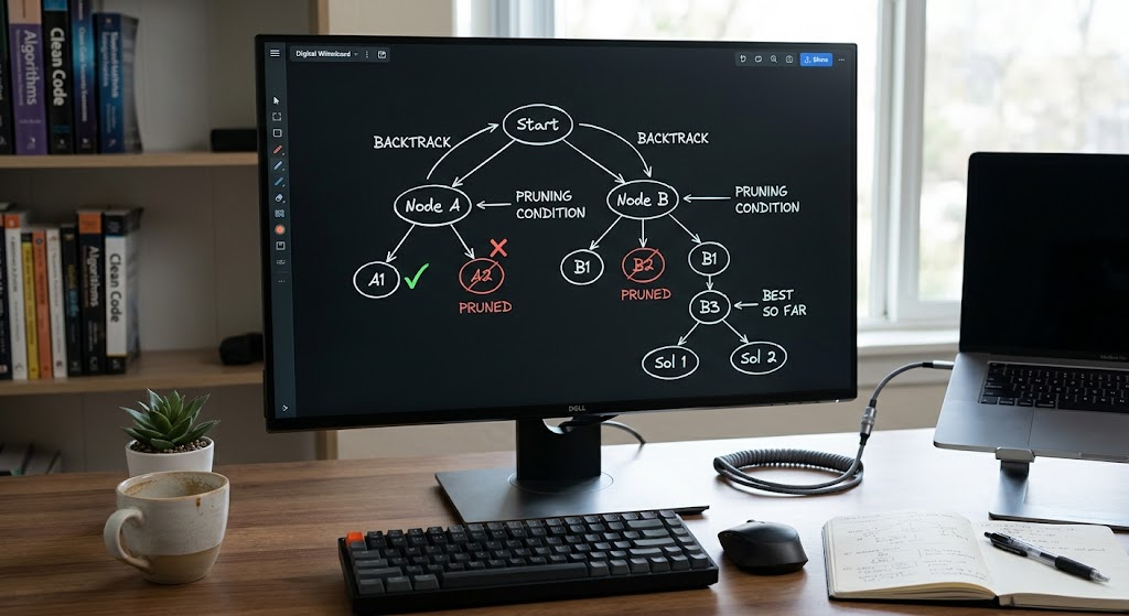
These are both algorithm design strategies for problems with multiple potential solutions. They search through potential solutions by using a state space tree. This represents partial solutions at each node, and the branches represent different decisions that can be made. Backtracking and branch and bound look at the progress made, and decide if the search should continue down a particular route. Both algorithms can help reduce unnecessary searches. However, backtracking is typically used to solve constraint satisfaction problems, where the aim is to find solutions that satisfy certain rules. Whereas, branch and bound is designed mainly for optimisation problems.
Pruning is used in both algorithms. This involves discarding branches of potential solutions based upon the information that is known. For example, if you are solving a puzzle and discover that any further numbers will not work due to previous choices not satisfying the constraints of the puzzle. Or if you are trying to optimize a delivery route and know that the estimated minimum cost of a certain route is higher than the best route found so far. This makes them both more practical than basic brute force searching.
Backtracking Algorithm
How does it work?
Backtracking is a method of creating a solution, by making a series of decisions. At each step, the algorithm will check if the partial solution satisfies the constraints of the problem. If the choice is valid then the next decision will be made. However, if the choice does not satisfy any of the constraints, or cannot be completed, then the decision is reversed and another choice is made. This will continue until a full solution is found, or all valid combinations have been searched. It is often implemented using a recursive method. The function will call itself to search through different combinations. This can give another level of decisions to make. Once the function has returned, the previous decision can be reversed.
Typically, backtracking will work by deciding what options are available for the current problem. It will then choose one option and check if it is valid. If it is valid then it will move onto the next option. However, if no valid options are available then it will backtrack to the previous decision and reverse the previous choice. Once all the required decisions have been made, the algorithm will realise that a solution has been found. This is useful as there will often be some constraints in the problem, so invalid combinations can be identified.
N Queens Problem
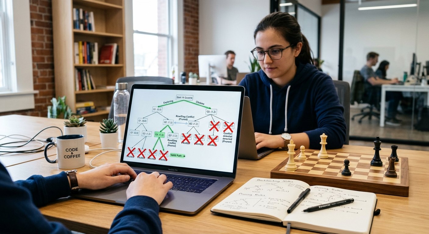
One of the most well known examples of backtracking is the ‘N Queens’ problem in computer science. This involves placing N queens on an N x N chess board. The queens will not be able to attack each other. In chess, queens can move horizontally, vertically and diagonally. Therefore, no queens can be placed in the same row, column or diagonal. A basic approach would involve creating different combinations of queens and seeing if they satisfy the constraints. However, this will involve a huge amount of combinations for larger boards. Using backtracking, the queens can be added one row at a time. Each time the algorithm will check if the new queen will be safe.
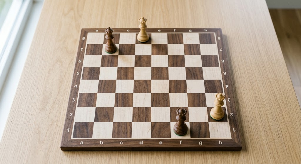
For example, if we are solving the 4 queens problem, the algorithm will place the first queen in a valid spot in the first row. It will then look at potential spots in the second row. Any spots that are in the same column or diagonal will be rejected. If a valid spot is found then it moves onto the third row. However, if there are no valid spots, the queen from the previous row will be removed and another spot tried. The advantage of this is that the algorithm will not waste time creating any invalid combinations. It will backtrack and try a different choice.
Solving Sudoku
Backtracking can be used practically to solve constraint satisfaction problems. A standard Sudoku puzzle has a 9×9 grid with 9 smaller 3×3 grids. The aim of this puzzle is to add numbers to the empty cells. The numbers must be between 1-9 and there cannot be any repeated numbers in the same row, column or 3×3 grid. Manually, you would try adding numbers to see if they fit. Using a computer, we can do this systematically with backtracking. The algorithm will look for empty cells and try adding numbers. It will then check if the number fits.
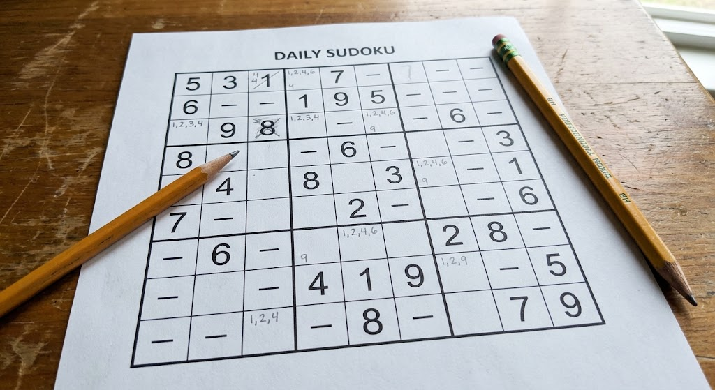
If there are no valid numbers to add to an empty cell, then it will know that the previous choice caused an issue. The algorithm will backtrack to the previous cell and remove the number. It will try another number. This will continue until the puzzle is solved. Backtracking can be used effectively to solve Sudoku. Often invalid number combinations can be identified. To improve performance, the cell with the least number of options can be chosen. This helps reduce unnecessary searching.
Applications of Backtracking
Backtracking can be useful in many areas of computer science. It can be used to solve graph colouring problems. This involves adding different colours to connected regions or vertices. It can be used to create permutations and combinations. It can also be used to solve word search problems, find paths in mazes and find solutions that satisfy scheduling constraints.
In software development it can also be used to solve configuration problems. For example, if a system is giving resources to different tasks, backtracking can be used to find a solution. This will discard any combinations of resources that don’t satisfy the constraints. It is very flexible and can therefore be useful wherever you need to find one or more valid combinations from a large selection of options.
Branch and Bound Algorithm
How does it work?
Branch and bound is typically used to solve optimization problems. Whereas some problems just require a valid solution, optimisation problems require the best solution to be identified. The algorithm will split the search into smaller sub problems. Bounds are calculated to show how promising each option may be. The algorithm will keep track of the best full solution found. This is often referred to as the incumbent solution. The algorithm will then compare the estimated potential of other partial solutions. If a partial solution will never improve the solution then it will be discarded.
Branching and bounding are the two main processes involved. Branching splits the problem into smaller options. Bounding calculates an estimated best solution for each partial solution. If we are trying to minimize the solution, a lower bound can be calculated. This gives an idea of the minimum cost to finish a particular branch. If this is higher than, or equal to the best full solution found then the branch can be discarded. If we are trying to maximize a solution, then an upper bound can be calculated. This will discard branches that cannot improve the current solution.
Travelling Salesperson Problem
An example of an optimisation problem that can be solved using the branch and bound algorithm is the Travelling Salesperson Problem. This involves finding the shortest route for a salesperson to visit a collection of cities once and return to the start. There will be some cost or distance between each of the cities. The aim is to find the route with the lowest overall cost. As the number of cities increases, the number of potential routes can increase significantly. Generally, for a problem with N cities, there will be (N-1)! / 2 unique routes in a complete symmetric distance graph. This can become impractical to check all routes for large problems.
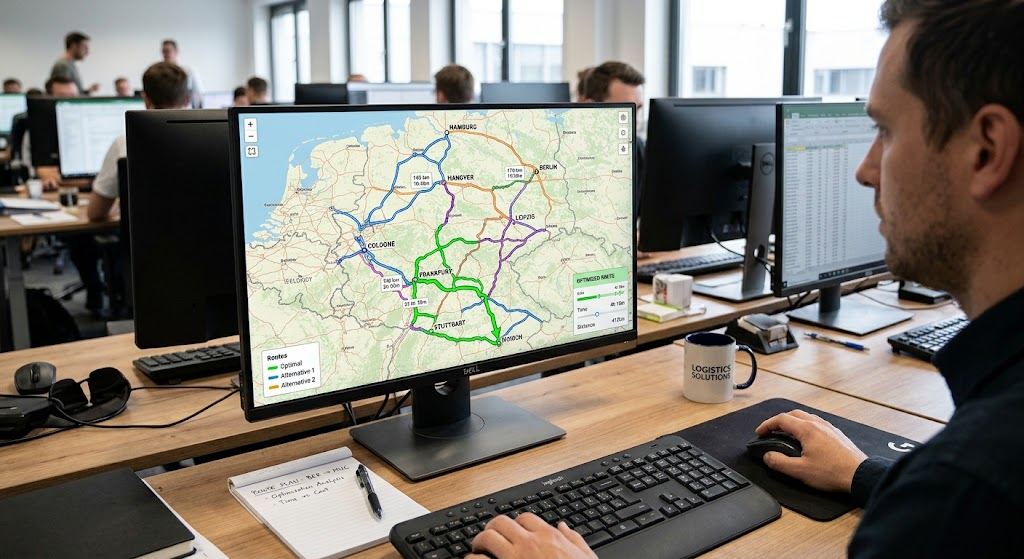
Imagine we have a salesperson to visit 5 cities. The algorithm will begin by looking at possible routes from the start city. It will calculate the cost of the partial route. It will then calculate the minimum extra cost needed to complete the route. If we have a partial route with a cost of 150 units, and we calculate the lower bound of this route to be 280 units. The best full route so far has a cost of 350 units, so this may be explored further as it could give a better solution. However if we have another partial route with a lower bound of 380 units, this can be discarded as it will not improve the solution.
Scheduling
Branch and bound can be used to help solve complex scheduling problems. This often involves finding the best way to order a collection of activities to minimise time, cost or resources. Many businesses, manufacturing companies and computing systems will have situations where different tasks have different processing requirements, deadlines and resource constraints.
For example, a manufacturing site may want to find the best order to complete a collection of production jobs. This will involve a limited number of machines. Different orders can give different completion times and costs. Branch and bound can be used to represent the different orders as branches in a search tree. Bounds can be calculated to show how much work is left to do. If a partial solution cannot improve on the best solution found so far then it can be discarded.
Resource allocation
Branch and bound can also be useful for resource allocation. Imagine you have a company with a limited budget. There are multiple projects to choose from. Each project will give a different expected benefit but will require a certain amount of investment. The aim is to select a collection of projects that will give the highest overall benefit without exceeding the budget.
Branch and bound can be used to find a solution. An upper bound can be calculated to show the maximum benefit that can be obtained from a partial solution. If the upper bound is less than an existing full solution, this can be discarded. This can allow us to find an optimal allocation without checking every combination. However, this will depend on how good the bounds are and how big the problem is.
Applications of Branch and Bound
Branch and bound can be used for many optimization problems in computer science, business and engineering. Common examples include the travelling salesperson problem, 0/1 knapsack problem, job scheduling, assignment problems and some types of network optimisation. For example, the knapsack problem involves selecting items with different values and weights.
You have a maximum weight capacity that you cannot exceed. The aim is to maximise the total value of your selected items. Branch and bound can calculate an estimate of the maximum value that can be obtained from a partial solution. This can discard combinations that will not improve on the best selection. It can also be useful for planning transport routes, allocating staff to tasks and organising production tasks where multiple conflicting options need to be considered.
Differences Between Backtracking and Branch and Bound
Although both algorithms use searching to find potential solutions, they have different aims. Backtracking aims to find solutions that satisfy a collection of constraints. If a partial solution does not satisfy a rule or cannot be completed then it will be discarded. Whereas, branch and bound aims to find an optimal solution. It will decide whether a branch can improve on the best solution found. Whilst both algorithms may use searching trees, recursion and pruning, they will not evaluate the solutions in the same way. Backtracking will evaluate whether a solution is valid. Branch and bound will evaluate whether a solution is competitive based upon an objective function and calculated bound.
| Feature | Backtracking | Branch and Bound |
| Main Aim | Find Valid Solutions | Find Optimal Solutions |
| Common Problems | Constraint Satisfaction | Optimisation |
| Pruning | Discard invalid/impossible partial solutions | Discard branches that will not improve the current solution |
| Evaluation | Evaluate if solution satisfies constraints | Calculate upper/lower bounds |
| Search | Typically uses depth first search | Can use depth first, breadth first or best first search |
| Memory | Often stores current path | May store multiple active nodes |
| Examples | N Queens and Sudoku | Travelling Salesperson and Knapsack |
| Main Aim | Satisfy Constraints | Optimise Measurable Solution |
Another difference is how they handle potential solutions. If only one solution is needed then a backtracking algorithm may stop once it finds a valid arrangement. Alternatively, it can continue searching to find all valid solutions. Branch and bound typically needs to compare solutions, as finding one solution will not guarantee that it is the best. It must keep track of an appropriate bound and continue searching until no branches can improve on the incumbent solution. This is an important consideration when deciding which algorithm to use. Developers should understand what type of solution they need for their problem.
Backtracking/Branch and Bound vs Brute Force
Brute force searching is a simple way to solve problems. It will search through every potential solution until it finds the answer. Whilst this is easy to understand and implement, it can become inefficient when there are a lot of potential solutions. For example, a program may generate different combinations of queens to solve the N Queens problem. Or for the travelling salesperson problem, it may generate different routes between cities and calculate the total distance. This may work for small examples but can become extremely large computationally.
Backtracking is an improvement on this as it will check constraints whilst creating a solution. For example, a brute force algorithm may generate full combinations of numbers to solve a Sudoku puzzle. Whereas backtracking will check each number as they are added. This will help discard any invalid solutions quickly. Branch and bound improves optimisation searching by using calculated bounds. This will discard partial solutions that will not improve on the current solution. For example, it will not complete every delivery route as it knows the minimum possible final cost of some partial routes will be too high. Both will reduce unnecessary work but will not guarantee quick solutions for every problem.
Advantages and Disadvantages of Both Algorithms
Advantages of Backtracking
One major advantage of using backtracking is that it can search through complex combinations in a structured way. As it uses recursion it can be quite easy to implement for problems with multiple decisions and clear constraints. Invalid partial solutions can be identified quickly.
Many implementations will require little extra memory as depth first search can be used. This can make it useful for learning exercises, puzzles and some software configuration problems. It is very effective when there are strict constraints that will help eliminate large sections of the search space.
Disadvantages of Backtracking
However, if there are many potential combinations and few strict constraints then backtracking can still require a lot of computational power. The time complexity can often be exponential or factorial depending on the problem. For example, Sudoku can have a very large search space when there are many empty cells. Permutation based problems can require factorial combinations to be searched.
If the decisions are not ordered well then many un-promising branches will be searched. Techniques such as constraint propagation, variable ordering and efficient validation can help improve performance, but the fundamental issue with every problem is that they can be computationally intensive. Backtracking will not always be efficient due to using pruning.
Benefits of Branch and Bound
A benefit of using branch and bound is that it can be used on optimisation problems that require an exact solution. Because partial solutions are bounded, it can greatly reduce the search space to find the true optimal solution. It is a flexible technique as developers can implement different searching strategies. For example, a depth-first search can reduce the amount of memory required, whereas a best-first search can help prioritize branches that have a higher estimated outcome.
It is a useful technique when attempting to solve problems related to transport, scheduling, manufacturing and resource allocation. Finding an improved arrangement can significantly increase the overall efficiency. If there are good bounds it can show great improvements over a brute force search.
Drawbacks of Branch and Bound
This technique relies heavily on the quality of the bounds. If there are poor bounds then many branches will not be pruned. The number of combinations can still be exponential or factorial in difficult optimization problems. Some implementations will require large amounts of memory as there will be multiple active nodes.
Calculating accurate bounds can add extra computational cost if the bounds are complicated. Therefore it cannot be guaranteed that this method will run quickly on any optimization problem. Developers will need to consider the size of the problem, memory available, the objective function and the quality of the bounds.
Computational Complexity
It is important to understand the computational complexity of a problem to know if backtracking or branch and bound will be a good option. Backtracking algorithms often have exponential or factorial computational complexity in the worst case. The number of combinations that may need to be checked can be very high. For example, a simple Sudoku solver can have an exponential search space based on the number of empty cells.
The N-Queens problem also has a rapidly increasing number of combinations. Branch and bound will have an exponential computational complexity in the worst case for many difficult optimisation problems like the travelling salesperson. However, good bounds can cause many combinations to be pruned. This depends on the nature of the problem.
Memory
A recursive backtracking algorithm will usually store the partial solution and the information needed to backtrack. This means that the amount of memory used is often dependent on the depth of the search. This will vary depending on the implementation. Branch and bound may require more memory.
Best-first search will use a priority queue to store multiple promising branches. This can be managed by using an appropriate search strategy, improving constraint checking, using efficient data structures and creating better bounds. It is also important to try different implementations with realistic sized problems as the complexity may not reflect how the algorithm will perform.
When to use Backtracking or Branch and Bound
The first thing to consider when choosing between backtracking and branch and bound is what the problem is looking for. Backtracking is generally a better choice when trying to find a solution that meets many constraints. Problems such as solving Sudoku, placing queens on a chessboard, generating valid combinations and colouring graphs will require backtracking. The algorithm will make decisions, check constraints and backtrack if an invalid arrangement is made. Backtracking works well if invalid combinations can be found early on. Developers will also need to consider if they want just one valid solution or all possible solutions.
Branch and bound is generally a better choice when trying to find the best possible solution to a problem. Problems that involve finding the minimal distance travelled, maximum profit, resource allocation and scheduling will often require comparing complete combinations to find the optimal solution. Branch and bound can be useful in this case as it calculates estimates to see if a partial solution can be better than the best solution so far. Ensure that the bounds are valid and effective. If it is too expensive to find an exact optimisation then other techniques such as approximation algorithms and heuristic searching may be more appropriate. The choice should depend on the requirements of the problem, expected size of the input, computational resources available and acceptable runtime.
Applications of Backtracking and Branch and Bound.
These techniques can be useful in real world applications. Backtracking can assist with finding valid combinations, valid schedules and solving puzzles. For example, an educational application that can generate or solve a Sudoku puzzle can use backtracking to try combinations of numbers. Software that can generate valid combinations of settings can also use backtracking to ensure they are not conflicting. Branch and bound can be useful in more complex scheduling problems. Optimisation can be used by transport companies to look at different delivery routes. Manufacturing organisations can use optimisation when organising manufacturing tasks. Search algorithms provide a structured way to solve problems with many conflicting combinations.
Both of these techniques can be useful for software engineers to understand how to approach solving computational problems. Rather than blindly searching through combinations, they can identify constraints, what to measure and when to abandon branches. This encourages better algorithm design as unnecessary operations can be minimised. However, real world applications should also consider varying inputs, processing constraints and that some optimization problems may become too large to use an exact search technique. Combining search techniques with heuristics, better data structures and approximation techniques can give more practical results. Understanding these techniques can help software engineers design programs to handle complex decision making and optimisation.
Conclusion
Backtracking and branch and bound are important techniques to use when designing algorithms. Backtracking builds up potential solutions and abandons any partial solutions that do not meet the conditions. It can be used to solve problems such as N-Queens, Sudoku, Graph Colouring and other constraint problems. Branch and bound is useful for optimisation as it breaks down the search space into smaller branches and calculates bounds to prune combinations that cannot improve on the best solution.
It is useful for problems such as the travelling salesperson, scheduling and resource allocation. Both techniques can reduce unnecessary searching, however they still have significant computational limitations in the worst case. Knowing the differences between the two, the benefits and drawbacks can help students and developers choose the correct technique to solve complex computational problems.