Introduction
Algorithms are the building blocks for modern computing, which allow computers to efficiently solve problems, process information, and perform tasks. Algorithms are used to interpret or process information on websites, to recommend products, and to help manage financial transactions, among other things; they control how software processes information and generates outcomes. But creating a working solution is just part of the programming task. Another important factor is the speed of execution and memory use, as well as the accuracy and the capacity of the algorithm to process (and process more and more) big volumes of data.
Algorithm design techniques include structured methods for establishing ways to solve complex problems in steps that can be managed by programmers. Developers will be able to use knowledge of techniques like Greedy Algorithms, Divide and Conquer, Dynamic Programming, Brute Force, Backtracking, and Recursion to solve problems in various ways. The methods help programmers think logically, develop problem-solving abilities, and develop software that is reliable and scalable as needs and tasks evolve.
What Are the Algorithm Design Techniques?
Algorithm Design Techniques are some systematic methods for designing algorithms to solve computational problems. Programmers do not try to solve all problems by trial and error; they have strategies to help them organize information, evaluate possible solutions and decide on the most efficient order of operations. The techniques all provide different approaches to a problem as a function of its structure, constraints and outcomes. For instance, divide and conquer can be useful in ordering a list of numbers, dynamic programming can be useful for selecting the most valuable subset of objects from a set with a restricted total cost, and a greedy strategy might be useful in selecting the largest possible subset of objects that can be purchased from a set with a restricted total cost.
Recognizing these distinctions enable developers to make decisions rather than following one approach to all tasks. Along with algorithm design, one must also consider the time complexity of an algorithm, i.e., how the time to run the algorithm changes based on the size of the input, and the space complexity of an algorithm, i.e., how much extra memory does the algorithm require.
Why Algorithm Design Matters
The performance and reliability of a computer program may be greatly affected by the selection of an appropriate algorithm. Say you have ten records, an obvious solution is great, but when you have millions of records, it’s not there for you to use. Efficient algorithms can minimize the need for unnecessary calculations, enhance response speed, and optimize the use of computing resources. They play a crucial role in scenarios that demand high-speed data access, such as large-scale databases, AI systems, scientific simulations, financial software, and real-time data processing applications.
Structured algorithms also tend to be easier to read, test and modify, and thus, easier to maintain. However, in all situations the fastest algorithm is not necessarily the best. In order to program a computer system, a programmer has to weigh a number of factors such as performance, complexity, memory usage, accuracy, and development time. The knowledge of basic design skills helps to assess these compromises and choose a solution that fulfills the technical design specifications as well as practical needs.
1. Brute Force: Solving Problems Directly by Examining Them
Brute force is one of the easiest algorithm design strategies. It refers to a systematic review of potential solutions to a problem, until a successful solution is found, or until all solutions that are relevant are considered. The algorithm takes a more straightforward path, typically simple to understand and implement, rather than using complicated shortcuts. For instance, if one of the programs requires to find a specific number in a list that isn’t sorted, then the program will need this.
A brute force approach can scan for the target starting with the first element until it gets to the end of the list. The algorithm can check up to 100 elements if the list has 100 elements. This technique is beneficial in smaller input scenarios, when a simple implementation is wanted, or when there is the need to have a reliable baseline to compare more complicated implementations. The greatest drawback is that it can involve many operations as the problem gets bigger and more complex.
Practical Example of Brute Force
Suppose that you are developing an app for shopping, and you need to find two items whose sum equals a given price. One of the simplest ways of checking if a given value can be formed using two products is by simply checking all the possible pairs. There are only 10 products in the list, so the number of pairs is reasonable. As the list expands, though, the number of comparisons will become quite large, since each product could be compared to numerous other products.
If there are n products in the list, then, a simple pair checking solution necessitates about n(n-1)/2n(n-1)/2 comparisons, which is O(n²). This approach is simple, but can be inefficient for large datasets. Furthermore, a programmer may make the program more efficient by employing a hash table that stores previously computed prices, so that in the usual case, the running time can be expected to be O(n). The simple example illustrates how to use brute force as a starting point, but also offers some optimisation potential.
Strengths and Weaknesses of Brute Force
The best feature of the brute force is its simplicity. It can be easily programmed using simple data structures and basic mathematical concepts, which makes it accessible for both beginners and small-scale computational problems. It is also useful if every possible solution has to be investigated to ensure the most optimal solution is reached. When the number of possibilities is growing exponentially or factorially, however, exhaustive examination may run into significant costs.
An example of this is attempting to find all possible combinations of a large number of objects, which may involve a great number of operations. In these cases, some other more efficient technique may be needed, like Divide and conquer, Dynamic programming or Backtracking with pruning. Brute force is still an essential problem solving method as it gives a clear baseline, can be used to compare alternative implementations, and can give the correct solution prior to any further optimization.
2. Divide and Conquer: Breaking Problems into Smaller Parts
Divide and conquer is an algorithm design method in which a large problem is broken into smaller subproblems, each of which is solved, and then the solutions are combined to get the solution to the original problem. Typically, the technique involves three steps – divide, conquer and combine. At the division stage the problem is divided into smaller parts. In the conquering phase, each part is solved, sometimes using the same algorithm recursively.
Lastly, the combination stage puts smaller solutions together to form the complete solution. This is useful when the subproblems can be solved independently and the results can be efficiently merged. It is widely used in sorting, searching, numerical computation and other large-sized data related applications. Divide and conquer can often give better performance than direct consideration of all possible solutions since the problem is broken down into “managable” parts.
Merge Sort as an Example
One of the fundamental examples of divide and conquer is merge sort. If a program needs to sort the numbers 42, 17, 8, 31, 24 into ascending order, how would it do this? In merge sort the list is recursively split into smaller lists of elements until each list is just a single element. The algorithm is already sorted and then it merges the lists in the proper order.
It continues to compare the smallest elements of the smaller lists and choose the next term until the two lists are joined. This process is repeated until all of the elements are in a single sorted list. The time complexity of merge sort is O(n log n) which is good for sorting large data sets. It has predictable performance and can be useful if efficiency is required, but it will likely need more memory to merge the lists in a conventional implementation.
Binary Search and Problem Reduction
This is another famous example of breaking a problem down into smaller problems: binary search. It searches for a specified value within a sorted array by comparing it with a value in the middle of the array. If the target is less than the middle, then the algorithm traverses the lower portion and if larger, the upper portion. If each comparison narrows down the search space by half, then about half of the elements will be rejected during each comparison.
Suppose that there is a list of 1,024 elements which is sorted. Then, the standard binary search will make approximately 11 comparisons in the worst case. This is much more efficient than checking each element of the array one by one in linear search. The binary search has complexity O(log n), provided that the data is sorted, and you can access the middle element efficiently. This example shows how divide and conquer can cut down on the work that is being done in unnecessary ways, and make the performance of common software operations better.
3. Greedy Algorithms: Taking the Greediest Next Step
A greedy algorithm proceeds to build a solution by choosing the step that seems optimal for the current state of the solution. Rather than looking at all the combinations, it makes a sub-optimal choice and keeps going until it arrives at a complete solution. This can be very effective as it eliminates the need to do any large searches and complex calculations. But a local optimum is not necessarily the global optimum. Greedy algorithms are correct for certain problems for which the structure of the problem ensures that the local optimal decisions can be used to determine a globally optimal solution.
Therefore, the programmers need to determine if the technique is suitable before using it. It is used in various applications, such as some scheduling problems, minimum spanning trees, and shortest-path calculations under certain conditions. Greedy methods tend to be appealing when it is possible to prove that they give correct solutions because they often have relatively easy to implement with low computational complexity.
Activity Choice: Practical Example
Suppose that a school computer laboratory needs to have different activities in one room with activity start and end times. The challenge is to schedule as much as possible, since the room is not able to accommodate activities simultaneously. This problem can be solved using a greedy algorithm: Sort the activities by their finish times, then pick the ones with the earliest finish time. It then chooses the next activity that can be completed as soon as possible and continues with the rest of the activities in the order they can be done, choosing each activity that begins after the last one selected has ended.
Selecting the activity that is earliest to finish with the least time to spare will ensure enough time is available for later activities. This approach yields an optimal schedule for the standard activity-selection problem, in which each activity has a fixed start time and end time and it is desired to select the maximum number of activities such that “no two activities overlap.” The example illustrates how, with a judicious choice of local rule, an efficient solution can be obtained without testing all schedules.
Dijkstra’s Algorithm and the Shortest-Path Problem
Greedy strategies are also used in graph algorithms. For instance, Dijkstra’s algorithm is used to calculate shortest paths from a starting vertex of a graph of non-negative weighted edges. For each step, it chooses the vertex with the smallest distance that has not yet been processed and adjusts the distances of the vertices adjacent to this vertex if a shorter path is found. This process gradually builds up shortest-path distances from the starting point.
It is applicable in navigation systems, network routing, and transportation systems where there are measurable costs or distances for connections. In general, Dijkstra’s algorithm is not correct, however, if negative weights are permitted the later negative edge can invalidate the earlier distance decision. This restriction also shows that greedy methods can be very useful depending on the properties and assumptions about the problem. Programmers need to be aware of those conditions before selecting an algorithm for the real world software.
4. Dynamic Programming: Solving Smaller Problems and Reusing the Solutions
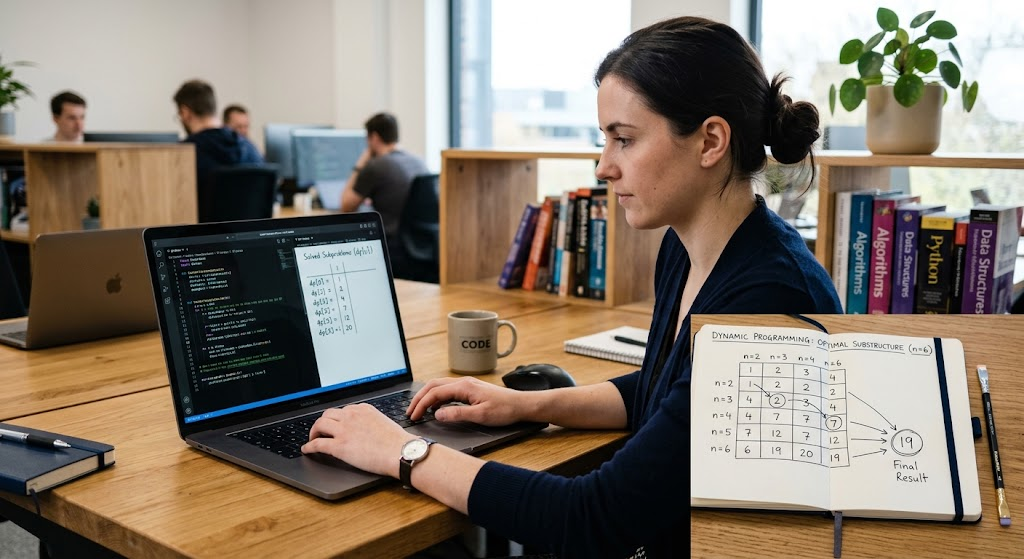
Dynamic programming is a method of solving problems by subdividing them into subproblems and saving the solutions to the subproblems and efficiently combining them to solve the original problem. When a problem has certain two characteristic properties overlapping subproblems and optimal substructure, it is particularly useful. Subproblems are smaller problems which are solved more than once in the solution process. Optimal substructure:Larger problems can be solved by combining appropriate solutions of smaller subproblems.
Dynamic programming prevents a program from doing extra work by using previously calculated results, and can reduce an inefficient recursive program to a much faster program. Depending on the problem, results may be stored in arrays, tables or other data structures. This method is often used in program optimization, counting, distributions of resources and sequence analysis, especially when the number of different subproblems is significantly less than the number of times these subproblems would be calculated otherwise.
Memoization and Tabulation
There are two methods of implementing dynamic programming: memoization and tabulation. Top down is memoization and starts with the original problem, recursively solves sub problems as necessary. Each result calculation is stored and future requests to that same result can be retrieved directly. Tabulation is a bottom-up approach that starts with the smallest subproblems, puts the answers to these subproblems in a table, and uses them to solve larger problems.
The two methods are designed to prevent unnecessary calculations, but the two methods are different in the way that they arrange the calculation. When only a limited number of subproblems are desired, memoization may be advantageous, but when the recursive call is deep, tabulation may be advantageous because it results in predictable performance without the need for expensive recursive calls. Depending on the problem structure, memory requirements, and the constraints for implementation, the best choice would be one of these.
Fibonacci Sequence: Practical Example
The Fibonacci sequence is a simple example of dynamic programming. Each number in this sequence is generated by adding up the two numbers that come before it, starting from the second number. The recursive implementation works quite simply, it computes the same previous values repeatedly, and the running time of this program increases exponentially with the desired position. To optimize the process, Fibonacci numbers that have already been calculated are stored and reused in dynamic programming whenever they are required.
For instance, after the fifth Fibonacci number is computed, the algorithm can use it without having to reconstruct the list of previous calculations. A bottom-up implementation can compute the first nn Fibonacci numbers in O(n) time, using O(n) extra space to store the entire sequence. The space required can be reduced to only O(1) if only the last two values are required. This gives an example of how recognising recurring work can lead to a significant increase in efficiency.
The Knapsack Problem: Practical Example
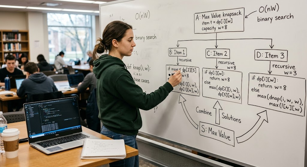
The knapsack problem is an example of how dynamic programming can aid in decision making with a finite resource. Suppose a student has a bag of a certain maximum weight that is to be used for a trip. Each item has a value and a weight and you want to choose some items to maximize the value for the bag’s capacity. If the greedy strategy uses the item with the maximum value first, it is possible that this item may take up too much room and not allow a better combination to be chosen. Dynamic programming can compute optimal solutions to small subsets of the items and weight capacities, and save optimal solutions for subproblems. With these results, the algorithm can be used to find the optimum combination, given the constraints. A common solution to the standard 0/1 knapsack problem is O(nW) time, which is a dynamic programming solution with nn items and WW when capacity is an integer. This is known as pseudo-polynomial time because it is dependent on the numerical capacity, not just the number of bits required to represent it.
See Wikipedia for a more extensive description of what is meant by dynamic programming. In order to write efficient programs, programmers should be aware of when repetitive calculations can be prevented, which helps them understand how this technique works. But DP is not a method to be used for every optimization problem. Its success relies on being able to represent the problem by a tractable set of overlapping subproblems and the ability to store the answers to the subproblems. If these conditions exist it can give an efficient trade off between solution quality and computation time.
5. Backtracking: Systematically Exploring Possibilities

Backtracking is an algorithm design method in which the algorithm explores the possible solutions step-by-step and when it is determined that the solution does not meet the constraints of the problem, they backtrack and try another solution. The algorithm backtracks to a previous choice and explores another possible choice. This is frequently done with recursion and can be seen as a search tree, with each branch being a choice.
Backtracking is especially beneficial for constraint satisfaction problems, puzzles, combinatorial search problems, and for problems that require a valid arrangement from a myriad of options. It can search a lot of candidate solutions in the worst case, but by discarding invalid partial solutions early can avoid a lot of unnecessary repetition of work. Thus its efficiency depends on the constraints of the problem, the order in which the choices are made and the effectiveness of the pruning rules.
A Practical Example: Solving Sudoku
A popular problem that can be solved via backtracking is Sudoku. The goal is to complete a 9×9 grid where every row, column and 3×3 box uses the digits 1 through 9 exactly once. The backtracking algorithm starts by finding an empty cell, and attempting to place a digit that isn’t “illegal,” in light of the existing digits in the row, column, and box. When the digit forms a partial arrangement, the algorithm moves on to the next empty cell.
If there is no legal move, then it goes back to the previous cell and makes another attempt. The algorithm is repeated until a complete valid arrangement is found, or until it is determined that such an arrangement is impossible under the conditions specified. Having constraints in place prevents the algorithm from pursuing any branches that will be invalid along the way. More sophisticated versions could choose the most constrained empty cell to fill first, thus limiting the amount of choices that may require consideration.
Backtracking in Combination Problems
Backtracking can also be used to solve problems with combinations, permutations, and allocation of resources. For instance, consider a set of programs that are required to create all possible sequences of the tasks that must make up the programs, while adhering to rules on which tasks appear next to each other. The algorithm can build the arrangement from the start, one decision at a time, discarding any partial arrangement that fails to meet a rule. Likewise, a maze-graph search could wander around trying to find an avenue through the maze, going around unnecessary walls and revisiting states.
They all have the same idea: develop a candidate solution step by step, test it and discard it if it doesn’t seem to be working toward an acceptable solution. Backtracking works well when there are constraints that allow us to cut off a lot of the search space. However, if there are only a few options that are eliminated in the initial stages, there can be an exponential number of possibilities left. Therefore, it is important for the programmer to take into account other optimization techniques (e.g., pruning, good decision ordering, etc.) when designing a backtracking algorithm.
6. Recursion: Solving a Problem in Smaller Copies of Itself
Recursion is a programming method where a function calls itself to solve a smaller instance of a problem or a simpler version of the problem. A recursive solution must have a base case that prevents any more recursion as well as a recursive case that takes the solution closer towards the base case. Otherwise, the function can run forever, leading to a stack overflow or other execution limit. Recursion is suitable for problems with a hierarchical or self-similar structure, such as traversing a tree, exploring a directory, implementing divide-and-conquer algorithms or performing some mathematical computations.
It can help make code more readable and easier to understand by breaking a complex task down into simpler parts of it. But recursion uses stack space and over-optimized recursion can repeat unnecessary calculations. Therefore, programmers should be responsible for making sure that each call moves toward termination and must reflect on the possibility of implementing the program iteratively, which may be more efficient or easier to maintain.
To Calculate a Factorial
The factorial of a non-negative integer n is the product of all the positive integers less than or equal to n, and is defined to be 1 when n is 0. Five factors are 5 times 4 times 3 times 2 times 1, or 120. One recursive factorial function could use the factorial of a number to define the factorial of the previous number. The base case is that if the function equals 0 or 1, the answer is 1.
The recursive calls will decrease the input until the base case is reached, then the results will be merged up as the function continues to return. It takes O(n) time and O(n) call stack to implement an input of size nn. While it is an excellent example of recursion, an iterative loop requires only one extra piece of data, and can be used in O(1) space if it is important to not use the stack or if the input data size is large.
Recursion and Its Relationship with Other Techniques
While recursive approaches can be part of a solution to a problem, as with other problem-solving methods, like greedy algorithms or dynamic programming, they are not always the best approach. Rather, it is an expression of calculation that can be applied in a number of algorithm design techniques. Both divide and conquer and backtracking involve recursive calls to explore different options in solving a smaller part of a problem. Dynamic programming can be implemented recursively by storing the results of previous computations, which are then re-used.
But using only recursion is not enough to ensure an efficient solution. There may be many subproblems with the same solution (as in the naive Fibonacci algorithm), or too many calls to functions (as in the recursive version of quicksort). Programmers need to be aware of the number of recursive calls, the size of each subproblem, and how much memory is used by the call stack. It is important to know when to use recursion and when to use memoization or iteration to make the recursive solution better.
7. Comparing Different Algorithm Design Techniques
All of the algorithm design techniques solve different classes of computational problems and the selection of an algorithm for a particular problem depends on the nature of the problem, its limits and requirements. Brute force is good for simple problems, simple inputs, but too many possibilities for larger problems. Divide and conquer algorithms break problems down into smaller subproblems and work well for merge sort, binary search, etc. When the problem can be proved to ensure that locally optimal decisions are globally optimal, then greedy algorithms can be very efficient. Useful for optimization and counting problems; Dynamic programming saves time by storing solutions to subproblems that are solved repeatedly. Backtracking is used to explore the candidate solutions and eliminate all the possible partial solutions that violate the constraints; this is useful for constraint-satisfaction problems. Recursion, on the other hand, offers a means of stating a problem in terms of smaller problems of the same type and is used by some of the other approaches.
Their main properties and application are summarized in the following table:
| Technique | Main Approach | Common Applications | Main Limitation |
| Brute force | Analyzes potential candidates first hand | Linear search, simple pairs checking. | May be slowed down as options grow |
| Divide and conquer | Splits a problem into subproblems and merges them | Explain two types of searching: Merger sort and binary search. | Results or dividing the problem can put an extra strain on the overhead. |
| Greedy algorithms | Makes the best decision based on a set rule, without delay | Under certain conditions, selection of activities is just like Dijkstra’s algorithm. | Not every local optimum is a global optimum. |
| Dynamic programming | Memorizes answers to previously encountered subproblems | Knapsack, Sequence problems, Fibonacci calculation | May need a lot of memory or many states |
| Backtracking | Looks for options and discards inadmissible partial solutions | Sudoku, mazes, constraints solving | The worst case running time may be exponential |
| Recursion | Uses calls to smaller copies of itself to solve a problem | Tree traversal, factorials, divide and conquer. | May waste stack space or repeat computations. |
Choosing the right Technique to Use
Choosing an algorithm design technique starts with understanding the problem, not by coding. Programmers should determine what they want to print, what the input constraints are, what the conditions for a “good” output are, and if there is any, an optimal output or not. If the input is small, and simplicity is the primary concern, then brute force can do the job. Divide and conquer might be a more efficient structure if the problem can be decomposed into independent subproblems. A greedy algorithm may be suitable if a good local decision rule can be shown to yield the optimal outcome.
If there is overlap of smaller problems and if the solutions to these problems can be used repeatedly, then dynamic programming can be considered. Backtracking might be more appropriate when exploring combinations with constraints. Any method which naturally breaks into repetitive small problems can be supported by recursion. Programmers can then analyze the time and space complexity of potential solutions, as well as conduct experiments on a variety of test sets and perform experiments with challenging or very large test sets.
8. Good Design of Efficient Algorithms
When designing an algorithm, more than just picking up a known method is needed. To start, the problem should be clearly defined, edge cases should be identified and the behavior of the solution should be confirmed. Then they should choose an appropriate data structure and decide if the algorithm should return an optimal solution or a valid one. Investigating time and space complexity is one way to determine the behavior of the solution with increasing input and testing is used to determine if the implementation is following the logic of the solution.
There are also some practical issues to take into account such as the amount of memory, size of input, restrictions in the programming language, and the cost of maintaining the code. A good algorithm for a small demonstration that doesn’t work in a large production database. Developers can construct correct and efficient solutions by using theoretical analysis and careful testing and measuring.
Analyze and Optimize
Time complexity is the number of operations the algorithm takes to execute based on the input size, and space complexity is the amount of memory that the algorithm uses based on the input size. A common way to describe an upper bound on this growth is big O notation, which enables a programmer to compare algorithms without being concerned about specific hardware or programming language. A linear search, for instance, has a time complexity of O(n) since the number of elements scanned could grow linearly as the size of the list increases.
Each step of binary search reduces the search space by half, making it efficient with a time complexity of O(log n). The nested loop solution can be O(n²) time and that can be costly for large inputs. But complexity analysis doesn’t cover all of the practical factors of performance, such as constant overhead, cache behavior and the quality of an implementation. Complexity analysis can be helpful in developers’ finding bottlenecks in their programs and in benchmarking programs when the performance is important in real life.
Test Edge Cases and Verify Correctness
An algorithm should give the correct answers when used with normal and unusual or even “borderline” inputs. For instance, a search function should be able to search an empty list, a value that is on the first position in the list, a value that is on the last position in the list, and a value that is not present on the list. A knapsack implementation should take two things into consideration: items that are too big to fit and no capacity at all. Recursive functions require base cases that do not lead to an infinite number of calls and the backtracking algorithms need to be able to recognize when a candidate solution is complete and when it is incorrect.
By testing these situations, bugs that may not be discovered during development are discovered. Programmers can also test both a new implementation and a simple brute force approach against a small set of randomly-chosen inputs, in the hopes that the reference implementation is reliable. This method can reveal errors in more complex algorithms and add to the trust that optimizations didn’t alter the necessary behavior.
Conclusion
The ability to solve computational problems correctly and efficiently is achieved by using the algorithm design techniques as a tool for the programmer. Brute force is a simple method of checking out possibilities, and divide and conquer breaks a problem into smaller subproblems. The strategy of solving the problem optimally at every step is referred to as greedy algorithm and dynamic programming helps to reduce computation time by storing the solution to the subproblems occurring multiple times in the problem.
Backtracking is used to search solutions which may fail due to constraints, while recursion is a way of representing a problem in terms of smaller instances of the same problem. Each technique has its own advantages and disadvantages and consequently, it is not appropriate for all computational problems. Developers can make informed decisions on design using the structure of a problem, analyzing its complexity, testing with edge cases, and comparing different solutions. These skills are crucial to the development of software that is dependable, maintainable and able to perform more complex calculations as needs grow.