Recurrence Relations
Recurrence relations are an essential tool in the study of discrete mathematics and are used to describe the evolution of mathematical sequences and processes in the computer. A recurrence relation is a way of defining each term of a sequence in terms of one or more previous terms. It can be helpful for a sequence to be following the same pattern or when a problem can be expressed as smaller versions of the problem. Recurrence relations are used in several fields of mathematics such as number theory, combinatorics, probability and mathematical modelling. They also have some important role to play in computer science as they give a systematic approach to analyzing recursive algorithms and estimating the computational complexity. Recurrence relations enable students to see patterns, create mathematical models, solve problems efficiently and appreciate how repeated calculations lead to larger outcomes.
Recurrence relations are very useful in computer science since many algorithms solve a problem by breaking it into smaller subproblems and then solving those subproblems. For instance, binary search keeps splitting the search space in half, and merge sort takes a sorted list and then merges it into smaller parts. Recurrence relations can be used to mathematically represent the number of operations that these algorithms perform. In the same way, sequences of numbers like the Fibonacci sequence are characterized by relationships between the terms of the sequence. The knowledge of building, analysing and solving recurrence relations forms a very solid basis for understanding algorithms, data structures, computational complexity and sophisticated mathematics.
What is a Recurrence Relation?
A recurrence relation is a mathematical equation which defines a sequence in terms of one or more previous terms. Explicit formula: a formula that gives a specific term based on its position.Recurrence relation: a relation that needs some information from previous terms to calculate the current term. Consider the sequence 2, 4, 6, 8, 10, and so on. The term can be expressed as a function of the previous term, an−1a_{n-1} using the recurrence relation an=an−1+2a_{n}=a_{n-1}+2. A starting value, like a1=2a_1=2, must be given to create the sequence. The recurrence relation then gives each term the value of the previous term plus 2. The idea of recurrence relations is that a mathematical pattern can be expressed as a rule which uses the previous results repeatedly, as in this example.
Addition, subtraction, multiplication, division, powers and more than one previous term can all be used in recurrence relations. There are some that only look back to the term before, and others that look back to several terms. For example, the sequence an=3an−1a_n=3a_{n-1} could be defined by saying that each term is three times the previous term. Another sequence can be defined recursively as an=an−1+an−2, which is defined by using the preceding two terms of the sequence. Recurrence relations can be complicated based on the mathematical structure, and the amount of previous terms applied to the relation. The usefulness of recurrence relations is that they can be used to describe, analyse and predict the behaviour of the recursive processes used in many mathematical sequences and algorithms in a systematic way.
Recursive Definitions and Initial Conditions
A recursive definition of a mathematical object is one that gives a rule for generating the objects after the first few and an initial value or values of the objects. Initial conditions in recurrence relations are important: The recurrence rule alone can be used to determine a unique sequence. For instance, if the relation an=an−1+5a_n=a_{n-1}+5 is given, then each term is 5 more than the preceding term but the first term has not been specified. If the first term is 1a_1=1, the first five terms of the resulting sequence are 1, 6, 11, 16, and . . . . . . . . . . For the starting value a_1=3, the sequence starts 3, 8, 13, 18, . . . . Both of the sequences have the same recurrence relation; however, they start with different initial values. This illustrates why it is necessary to have sufficient initial information in a complete recursive definition to establish the sequence.
Another role of initial conditions in recursive computer programs is crucial. A recursive function is a function which calls itself in order to solve smaller instances of a problem. Typically these functions have a base case that stops the recursive function and a recursive case that brings the problem closer to the base case. For instance, the factorial of a positive integer nn can be defined as 0!=10!=1, and n!=n(n-1)!n!=n(n-1)! for n≥1n\geq 1. The base case defines the factorial of 0 as zero and the recursive rule defines each positive factorial as the product of the previous one and the number. Consequently, 4!=4×3×2×1=244!=4\times3\times2\times1=24. The recursive definition would otherwise not terminate, but instead keep going on forever. Base cases and initial conditions are thus a critical part of mathematical recurrence relations and recursive programming alike.
Types of Recurrence Relations
Recurrence relations can be categorized based on: their mathematical form, the previous terms they involve, and whether the previous terms are linear or nonlinear. A common class is linear recurrence relation, where only the first power of the previous terms is used and they are not multiplied together. For instance, an=4an−1−3an−2a_n = 4a_{n-1}-3a_{n-2} is linear because the terms that are previous in the sequence are linearly represented. A nonlinear recurrence relation, on the other hand, can contain squared terms or products of previous terms, or other nonlinear expressions. For example, the previous term is squared to produce an=an−12+1a_n = a_{n-1}^2 + 1, which is nonlinear. This distinction is important since some mathematical methods are appropriate for certain kinds of recurrence relations. Linear recurrence relations with constant coefficients are typically solved by characteristic equations, while nonlinear relations can be solved numerically, by approximation or special methods.
A second major difference between homogeneous recurrence relations and nonhomogeneous recurrence relations is that homogeneous relations can be solved using only a single recurrence relation, whereas the latter require two. A homogeneous linear recurrence relation is a recurrence relation in which each term is a multiple of the preceding terms, for example, an=2an−1+an−2a_n = 2a_{n-1}+a_{n-2}. A nonhomogeneous recurrence relation has an extra term that is not a function of the values of the sequence, e.g. a_n=2a_{n-1}+3. Recurrence relations can also be ordered by the number of terms that need to be known to determine the next term. The first order and second order recurrence relations are those that depend on one and two previous terms, respectively. Knowing these classifications can aid students in determining a structure of a recurrence relation before choosing an appropriate method to solve it. It also offers a basis for distinguishing between the mathematical definitions of sequences and those of the recurrences that are applied to the analysis of computational processes.
Recurrence Relations – Methods for Solving
There are a few different methods to solve a recurrence relation, depending on the type of recurrence relation and what information is available. One of the easiest is the iterative method (also known as repeated substitution). This approach consists of expanding the recurrence relation a number of times, until a familiar pattern emerges. Consider an=an−1+3a_n=a_{n-1}+3, with a1=2a_1=2. Repeated substitution gives a2=2+3=5a_2=2+3=5, a3=5+3=8a_3=5+3=8, and a4=8+3=11a_4=8+3=11. If this continues, then each term is 3 more than the previous term. The explicit formula is an=2+3(n−1)=3n−1a_n=2+3(n-1)=3n-1. Simple recurrence relations and for a preliminary understanding of the behavior of a sequence are good cases for using iteration. But, for complex relations, repeatedly calculating the terms may be inefficient, so there are more systematic approaches needed.
One method is the substitution method: Make an educated guess for a solution and then prove it by either mathematical induction or algebraic manipulation. For example, suppose a recurrence relation is T(n)=T(n−1)+2nT(n)=T(n-1)+2n, with T(0)=0T(0)=0. Expanding the relation produces T(n)=2+4+6+⋯+2nT(n)=2+4+6+\cdots+2n. This expression can be rewritten as T(n)=2(1+2+⋯+n)T(n)=2(1+2+\cdots+n). Using the familiar sum formula 1+2+⋯+n=n(n+1)/21+2+\cdots+n=n(n+1)/2, we obtain T(n)=n(n+1)T(n)=n(n+1). It is found that the sequence is quadratic as its value is proportional to n^2n^2 for large n. Other methods are characteristic equations, generating functions, and the master theorem, which is applicable to some divide and conquer algorithm recurrences. The proper technique will depend on the structure of the recurrence, the form of the solution desired, and whether it is an exact solution or an estimate of the growth behavior.
Understanding Characteristic Equations
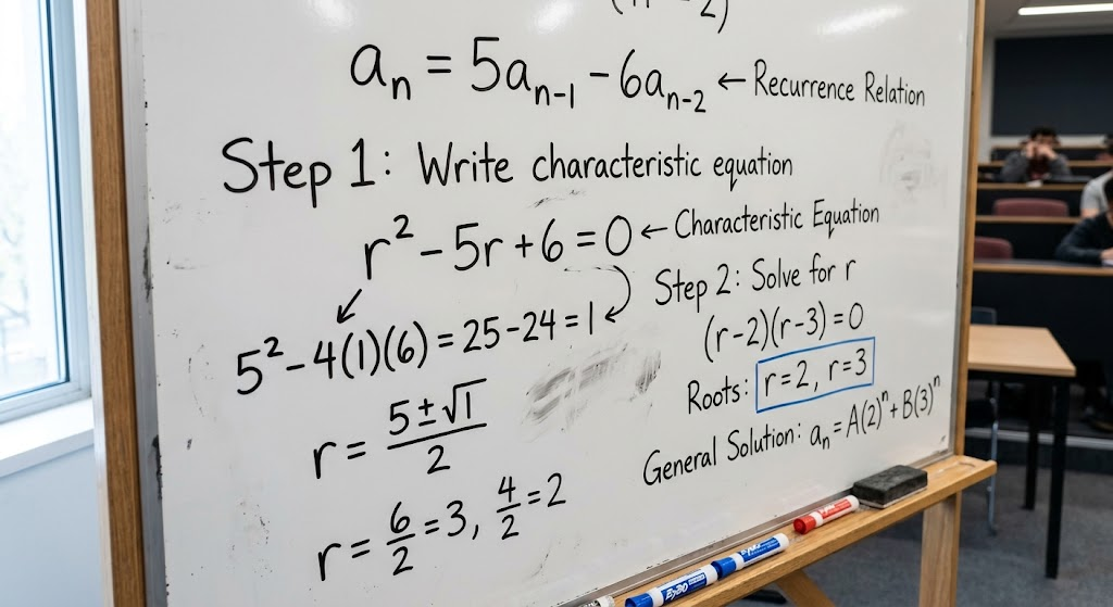
The characteristic equation method is a systematic procedure for solving a large number of linear homogeneous recurrence relations of constant coefficients. Suppose that an is a second-order recurrence relation in the form: a_n=pa_{n-1}+qa_{n-2}where pp and qq are constants. If we assume that the given sequence is of the form an=rna_n=r^n, where rr is a constant to be determined, then we can find a solution. Substituting this expression into the recurrence relation yields rn=prn−1+qrn−2r^n=p r^{n-1} + q r^{n-2}. If possible, factor out rn−2r^n-2, to get the characteristic equation r2−pr−q=0r^2-pr-q=0. Substituting values for rr into this quadratic equation will yield possible values for rr; these will then be used to build the general solution. This technique can be used to convert a recursive formula into an algebraic one, allowing us to find a formula for the sequence without computing each term.
The characteristic equation method is especially useful in solving linear recurrence, such as linear recurrence with constant coefficients. For example, consider an=5an−1−6an−2a_n=5a_{n-1}-6a_{n-2}, with initial conditions a0=2a_0=2 and a1=5a_1=5. Assume that rna_n=r^n gives the characteristic equation r2-5r+6=0r^2-5r+6=0. Factoring produces (r−2)(r−3)=0(r-2)(r-3)=0, so the roots are r=2r=2 and r=3r=3. The roots are different and the general solution is an=A2n+B3na_n=A2^n+B3^n where AA and BB are constants that depend on the initial conditions. Substituting a0=2a_0=2 gives A+B=2A+B=2, while substituting a1=5a_1=5 gives 2A+3B=52A+3B=5. The solution to these equations is A=1A=1 and B=1B=1. Thus, the explicit solution is an = 2n + 3na_n = 2^n + 3^n, and this would generate the original sequence, showing how characteristic equations give an explicit solution.
A Worked Example on Fibonacci Sequence
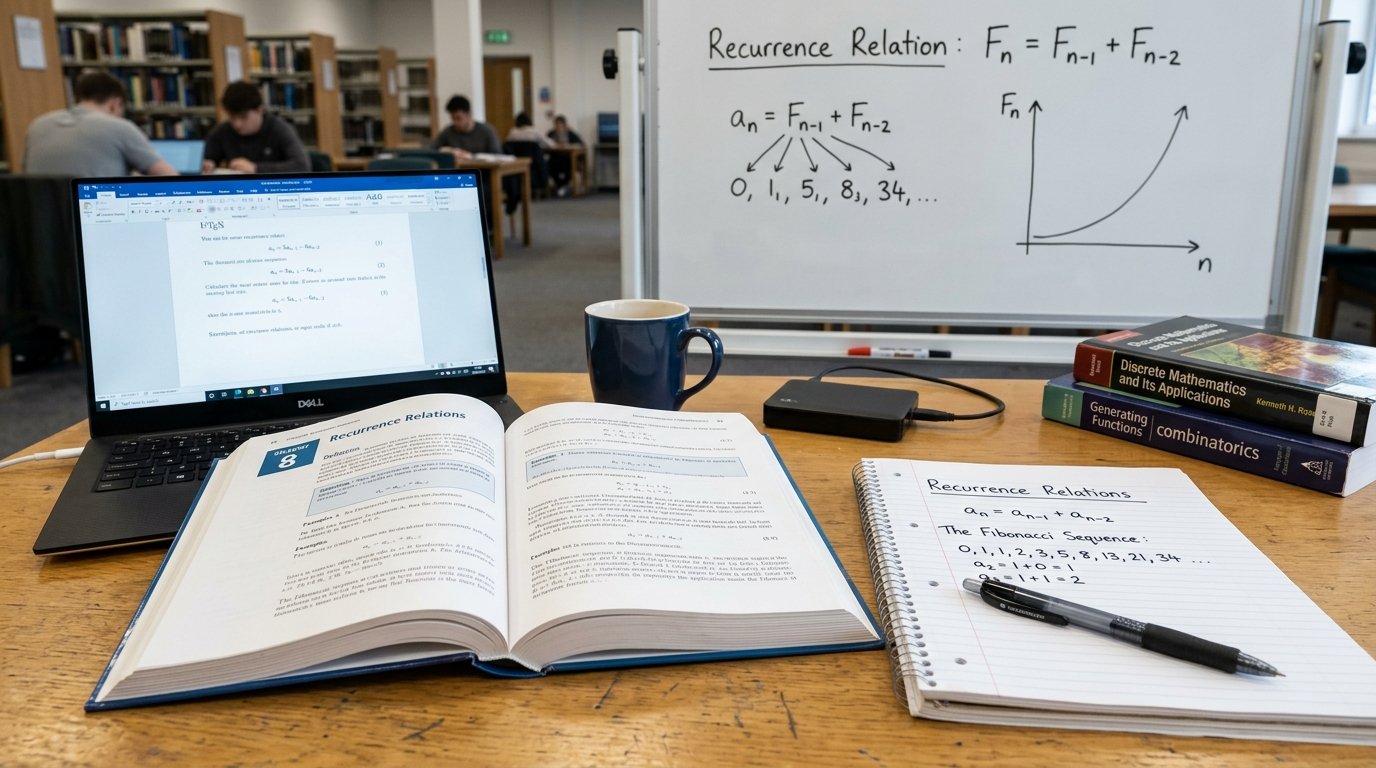
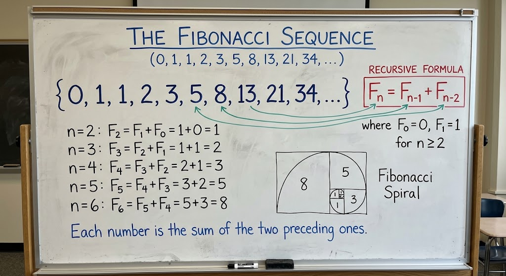
One of the most popular examples of a recurrence relation is the Fibonacci sequence. It starts with the values F0 = 0 and F1 = 1 and each term after the first is the sum of the previous two terms. Its recurrence relation is Fn=Fn−1+Fn−2F_n=F_{n-1}+F_{n-2} for n≥2n\geq2. Using this rule, the first several terms are 0, 1, 1, 2, 3, 5, 8, 13, 21, and 34. Each term of this sequence depends on the previous two terms, and as such, a simple recursive rule can produce an infinite sequence. The Fibonacci sequence is also useful for the purposes of teaching recurrence relations, since it is easy to understand, but it also illustrates the need for initial conditions, recursive computation and mathematical pattern recognition.
A characteristic equation can also be used to solve the Fibonacci sequence. The solution for Fn=rnF_n=r^n is r^2-r-1=0. Applying the quadratic formula gives the roots r=(1+5)/2r=(1+\sqrt5)/2 and r=(1−5)/2r=(1-\sqrt5)/2. These roots are often represented by the symbols ϕ\phi and ψ\psi, respectively. Using this, it is found that the resulting explicit formula is Fn=(ϕn−ψn)/5F_n=(\phi^n-\psi^n)/\sqrt5. This formula is called Binet’s formula and is used to represent Fibonacci numbers directly in terms of n. While recursive calculation is useful for computing the first few, the explicit formula also gives some other mathematical properties of the sequence. Fibonacci numbers have applications in combinatorics, mathematical models and some descriptions of natural patterns. The sequence is also a good example of how simple rules relate to more mathematical entities.
Recurrence Relations in Computer Science
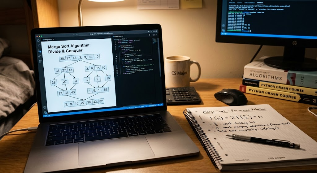
Recurrence Relations in Computer Science are used in many different ways.Many of the algorithms used in computer science require repeated operations or smaller subproblems to solve a problem, making recurrence relations a central role in computer science. Recursive algorithms often call themselves with smaller arguments, and recurrence relations give a mathematical formula for the running time of recursive algorithms as the size of their argument grows. For instance, suppose that one routine examines a list, takes action on the first element in the list, and then calls another routine to process the rest of the list. The work performed by this routine might be recursive in the first routine, with the remainder of the work being done by another recursive routine, but involving a constant amount of work per call to the first routine. The recursive definition for the first routine might be of the form T(n) = T(n-1) + cT(n) = T(n-1) + c, where c is some constant amount of work per call to the first routine. If the base case runs in a constant time, then solving this relation will yield linear time, O(n)O(n). This notation tells us what happens to the running time as the size of the input increases. A mathematical model of recursive behavior can be used to evaluate and compare algorithms, to find inefficiencies, and to select appropriate algorithms to solve computational problems.
Recurrence relations are also used in analysing divide-and-conquer algorithms, both of which divide a large problem into smaller subproblems and solve them and then merge their solutions. One of the traditional examples is merge sort. It splits the array into two roughly equal parts, sorts each part recursively, and combines the sorted parts into a single array. It takes 2T(n/2)2T(n/2) to sort the two halves and cncn to merge them, which gives its running time of T(n) = 2T(n/2) + cnT(n) = 2T(n/2) + cn. The base case is constant and the recurrence is O(nlogn). The recurrence relation is the reason that merge sort is more efficient than a simple quadratic-time sorting algorithm for sufficiently large inputs. It also shows that the analysis of algorithms needs to take into consideration not only recursive calls, but also the extra amount of work done at each level of the computation.
Recurrence Relations – Binary Search and Data Structures
Another major example of recurrence relations in algorithm analysis is that of binary search. An algorithm that uses comparison of the target to the middle element in a sorted collection to find the target value. If the target is not found right away, binary search discards around half of the space it is going to search next, and continues with the right half. It has a running time of T(n) = T(n/2) + cT(n) = T(n/2) + c, where nn is the number of elements and cc is the constant time it takes to compare elements and choose a new search interval. The recurrence has a logarithmic solution of T(n)=O(logn)T(n) = O(\log n), indicating that there are relatively few steps as the collection grows in size. For instance, with binary searching, a search space of 1024 elements can become reduced to one element in approximately ten halvings. This is the efficiency of the binary search that is useful when the data is sorted and elements can be accessed at random.
Recurrence relations also have practical applications in data structures, such as those with recursive traversal or repeated subdivision. For example, a binary tree can have nodes with the left and right child nodes. Recursively traversing a binary tree is often done by algorithms that process a node and then call themselves on the children of that node. Total running time will be a function of the number of nodes and the work performed at each node. In a balanced tree, operations like searching may be able to be done in logarithmic time, since the height will grow proportionately to log n log n nodes in the tree. A tree may on the other hand be unbalanced like a linked list, where some operations take linear time. Recurrence relations help describe these differences by relating the cost of processing a tree to the costs of processing its subtrees. They thus facilitate the study of traversals of a tree, recursive searches, and performance properties of important data structures.
The Master Theorem and Divide and Conquer Problems
A very popular formula that solves a specific kind of recurrence relation for a class of divide and conquer algorithms is the master theorem. These relations typically are of the form T(n) = aT(n/b) + f(n)T(n) = aT(n/b) + f(n), where aa is the number of recursive subproblems, n/bn/b is the approximate size of each subproblem, and f(n)f(n) is the amount of work performed outside recursive calls. The theorem compares the growth of f(n)f(n) to the quantity nlog_ban^{\log_b a} which is an important measure of the total contribution from the recursive subproblems. The theorem gives conditions for the recursive work or the extra work at each level or both to dominate the solution to the recurrence. This technique is useful because it can determine the asymptotic running time without having to expand the recurrence relation for a long time.
Write a recurrence for merge sort: T(n)=2T(n/2)+cnT(n) = 2T(n/2) + cn. Here, a=2a=2, b=2b=2, and f(n)=cnf(n)=cn. The comparison term is nlog22=nn^{\log_2 2}=n so the additional work cncn have the same asymptotic growth as the comparison term. Under the corresponding case of the master theorem, the solution is T(n)=Θ(nlogn)T(n)=\Theta(n\log n). The tight asymptotic bound of Θ(nlogn)\Theta(n\log n) means that for sufficiently large n, the running time is on the order of nlognn\log n. The Master Theorem can be applied to many common divide and conquer algorithms, but not all recurrence relations. Other special techniques are needed for some problems, such as iteration, substitution, recursion trees, and characteristic equations. It is a crucial part of mathematical or algorithmic problem solving to identify the correct approach.
Advantages and Disadvantages of Recurrence Relations
There are pros and cons to recurrence relations. A strong advantage to recurrence relations is that they allow us to describe repeated processes in a concise and comprehensible mathematical manner. A recurrence relation is another way to describe an algorithm by describing a rule for the whole algorithm without enumerating a long list of sequence values. This helps to see patterns, develop an explicit formula, and provide estimates for the resources needed by algorithms. The other advantage of recurrence relations is that they can be used to represent a large number of situations including numerical sequences, recursive functions, trees and divide-and-conquer calculations. They are used in conjunction with other tools like characteristic equations, mathematical induction, and the master theorem, to gain insight into the behavior of systems as their inputs or time steps grow. They have been utilized in the field of discrete mathematics, fostering analytical skills, and bridging the gap between abstract mathematical concepts and real-world computational challenges.
Although these are advantages, recurrence relations are not without their drawbacks. Not all recurrence relations have obvious closed form solutions by means of elementary algebra and some nonlinear relations may not have simple closed form solutions. If there is a solution, it may be hard to find, or involve a lot of math and/or advanced techniques. Recurrence relations are also sensitive to the level of accuracy in the computational model with which they are constructed in algorithm analysis. An analysis that fails to account for certain operations, memory usage, or worst case versus best case scenarios can lead to an estimate which doesn’t adequately reflect the algorithm’s actual performance. In addition, asymptotic notation deals with growth as the input size grows to large values and is not necessarily an accurate predictor of actual run times for small inputs. Therefore, it is important that recurrence relations are applied with good reasoning, sensible assumptions and, where needed, experimental evaluation of algorithms.
Conclusion
Recurrence relations are among the most basic tools of discrete mathematics in that they can be used to describe a sequence and repeated processes by means of a relationship between previous and current values. An entire sequence can be defined by using a recurrence rule and appropriate initial conditions. There are various methods for solving recurrence relations, depending on the type of relation.There are several rules to solve recurrence relations, such as iterative method, substitution, characteristic equations, generating functions, and the master theorem. The characteristic equation method is particularly useful for many linear homogeneous recurrence relations with constant coefficients and the master theorem is a useful tool for analyzing some common divide and conquer algorithms.
A few examples, like the Fibonacci sequence, binary search, and merge sort, illustrate how the concepts of recurrence relations relate mathematical concepts to actual computation. By mastering these ideas, students can identify patterns and come up with mathematical solutions, assess the efficiency of the algorithms they create, and create better problem-solving strategies. For this reason, recurrence relations continue to be a fundamental and important subject in discrete mathematics, computer science, data structures and algorithm design.