
Introduction
Whether calculating the shortest route between two addresses or suggesting products, making social media connections or organizing communication networks, computers process huge quantities of information every day. A great deal of these activities require knowledge of relationships among various objects but not necessarily relationships among various pieces of information. These relationships often can be expressed in graph algorithms, which also can be used to solve problems with connected data.
Graphs are a data structure which contain vertices (also known as nodes) and edges (which are the connections between the vertices). For instance, a road network could be modeled as a graph in which towns or cities are vertices and roads are edges. These relationships can be used to find the relationship between two locations, to find possible routes, to limit the movement between two locations, and to find efficient ways to organize a network. Graph algorithms are therefore a vital aspect of computer science that can help to solve problems involving relationships, movement, connectivity, and optimization.
What Are Graph Algorithms?
Graph algorithms are a step-by-step approach to the analysis, exploration and examination of a graph to address specific problems. These algorithms can be used for computers to search for information, find relationships between objects, compute shortest path between points, or find the cheapest path between points. Graph algorithms are designed to work with the relationships between elements rather than with the elements themselves that are set up in a list, as algorithms tend to do. Consider a social network containing thousands of users.
Every user can be modeled as a vertex, and friendship (or any relationships) can be modeled as an edge. A graph algorithm might be useful to identify mutual friends, whether two users are connected by other users, or groups with strong relations. In the same way, an online shopping site can visualize products and customer preferences as interrelated data to boost suggestions. The algorithm employed would vary according to the problem to be solved, the graph structure and the nature of information that can be associated with the graph’s links.
Understanding Graph Terminology
To discuss individual algorithms, it is important to discuss the basic concepts involved in describing graphs. A vertex is an object or location in a network, a person or other identifiable entity, and an edge is a relationship or connection between two vertices. For example, in a delivery network, the vertices can represent a warehouse and a delivery destination, and the edges can represent a road between them. A graph can also have a path defined as a sequence of connected vertices that can be used to go from one vertex to another.
A cycle is a path that returns to the starting vertex after being through other vertices. A vertex of an undirected graph is called of degree k if the vertex has k edges adjacent to it. In a directed graph, the number of edges coming into a vertex is known as the in-degree of that vertex, and the number of edges going out of a vertex is known as the out-degree of that vertex. They can be used to accurately describe network structures and to understand how information or movement can flow through them, which is useful for programmers. They also form the basis to select and apply suitable graph algorithms.
Directed and Undirected Graphs
There are two types of graph: a directed graph and an undirected graph. An undirected graph is a graph in which an edge denotes a mutual relationship. If two individuals are friends with each other on a platform that defines friendship as bi-directional, it can be represented as an undirected edge. Likewise, if travel is allowed two ways between two towns, then an undirected edge is used to represent the two-way road. In a directed graph, however, there are edges that go from one vertex to another, and that means that the relationship has a direction.
Links on a website is a good example, as one page can link to another page, but the latter isn’t linked to the first page. Directed graphs can also be used to model certain relationships and communication flows that are not bidirectional. It is important which type of graph is chosen, as this will determine the type of connections an algorithm will be able to access. If a directed relationship is treated as undirected, it may cause a program to believe there is a place where it can move when in reality there is not.
Weighted and Unweighted Graphs
Another difference is whether the weights of the edges can be nonzero. An unweighted graph is a graph that is not costed with numbers for each edge. In this case, the algorithm could be based on the number of connections that are needed to reach a destination. A Weighted graph assigns a value to each edge, which is used to denote some information like distance, travel time, financial cost or network delay. A road network can, for instance, include the weight of each road as the length of the road in kilometres.
Alternatively, a delivery system could use the estimated travel time or fuel cost as the weight. Different weights can be used to get different preferred routes, and the meaning of a weight is problem dependent. Roads that are not on a path may be much longer or busier than the roads that are on the path, making the path not necessarily the fastest. Therefore, knowing whether a graph is weighted or unweighted is important in determining which algorithm to use. Breadth-first search is more useful in unweighted graphs for finding paths with the fewest edges, and Dijkstra’s shortest-path algorithm allows for non-negative edge weights on the graph.
How to Represent a Graph in a Computer
In order to process a graph, computers must have an organized way of storing the vertices and the edges. Adjacency lists and adjacency matrices are two popular representations. An adjacency list is a collection of neighbours of each vertex and can be used to find vertices that are directly connected to a given vertex. For instance, if a town is linked to three other towns, you will have a list of the 3 towns that are neighbours. This representation is typically space efficient in the case of a sparse graph, where there are relatively few edges in relation to the number of possible edges.
An adjacency matrix is a two dimensional matrix whose elements are 0 or 1 indicating whether two vertices are connected in the graph or not. The entry shows whether or not there is an edge between the corresponding vertices, and can contain its weight. Use matrices for a graph with lots of graph connections or a program that checks regularly for a specific graph connection. But it can be memory intensive for big graphs. These representations can be chosen according to the size and density of a network, the amount of memory available and the most common operations carried out by the program.
Breadth-First Search: Exploring Connections Level by Level
BFS (Breadth First Search), also known as BFS, is a graph traversal technique that traverses vertices of a graph by level, starting from a given starting vertex. BFS does not visit the same vertex twice for a given source, and it visits the immediate neighbours of the source before vertices next to the immediate neighbours and so on. The algorithm usually relies on a queue, a data structure that processes items in the order that they are inserted. If a vertex is found, it is placed in visited and the unvisited neighbours placed in the queue.
When there are cycles in a graph, it is important for the algorithm to remember which vertices have already been processed to avoid processing them twice. BFS can be used to check whether one vertex can reach another in an unweighted graph, and to discover the shortest paths between vertices in such a graph. BFS can be used in some social networking applications to find the minimum number of steps needed to connect two users in the network. The systemicity makes it useful for analyzing networks where the cost of connections is not as significant as the number of connections.
A Practical Example of Breadth-First Search
In BFS, starting from A, A is visited and B and C are added to the queue. B is visited and D added to the queue. C is visited and E added to the queue. It then works out B and C, before heading to its new neighbours D and E. The traversal thus visits nearby vertices first and then further ones in the network. Each connection will take one step, so BFS will be able to find that D is two steps from A, via B, and E is two steps from A via C.
When all edges have the same cost this property is useful for determining the minimum number of links required to connect two points in the algorithm. In real systems, BFS can be used for finding neighbors, exploring computer networks, finding potential links among web pages and studying the structure of unweighted graphs. When the edges have different distances or costs, however, BFS doesn’t necessarily find the cheapest path because it does not take into account the weights of the edges.
Depth-First Search: Exploring One Path at a Time
Another graph traversal algorithm, called depth-first search (DFS), traverses a graph differently from BFS. In DFS, instead of searching all the adjacent vertices first, it takes one of the available paths and proceeds as far as it can from a vertex and then goes back to the previous vertex and searches another path. This is called back tracking. One can use recursion or a stack to implement the DFS. It does this by keeping a record of visited vertices, similar to BFS, which will prevent redundant exploration and infinite cycles if there are cycles.
DFS can be applied to find connected components, cycles, detect if there is a path, check relationships in complex networks, etc. For instance, a program that checks for the dependency between the software components uses DFS to explore the dependency between two components. It can also be used to explore the structure of folders, navigate mazes, or maps with connected regions. DFS can discover a path between any two vertices if such a path exists but does not guarantee that the path will have the fewest edges or the lowest total cost.
What Is DFS and How Does It Work Using an Example?
DFS starting at A will visit B, then D, and then back to A since it can’t go any further on that branch. It can then explore C and proceed to E. The possible traversal sequence is A, B, D, C, E, or any other sequence because of the way neighbours are stored and chosen. This is an example of how DFS explores one branch and then goes back to explore another branch. In a large graph, this approach can be useful for detecting cycles in a graph or for determining if a graph has cycles at all or if all vertices are reachable.
The DFS is also employed in other more sophisticated algorithms such as topological sorting and strongly connected components in directed graphs. Its effectiveness depends on its application and the graph structure. Recursive implementations might have a call stack limit on very deep graphs, an iterative implementation using an explicit stack could be more suitable.

Dijkstra’s Shortest-Path Algorithm
Dijkstra’s shortest path algorithm is one of the most famous graph algorithms, that finds shortest-paths in a weighted graph with non-negative edge weights. It is especially helpful when distances, travel times or costs are not the same for the connections. The algorithm first assigns a distance of zero to the initial vertex and sets the distance to other vertices to some value initially unknown or infinite. It will always choose the smallest known distance vertex that hasn’t been processed and it will look at adjacent vertices.
If the cost of travelling through the selected vertex is less to a neighbour than it was previously, the algorithm changes the cost of that neighbour. This is known as relaxing. The algorithm proceeds until the required vertices are visited, or a suitable implementation reaches the destination. Dijkstra’s algorithm finds a better path through a weighted network by comparing the cost of the connections (not just how many). It is used widely in computer science, and is important for grasping route planning and network optimization.
How Dijkstra’s Algorithm Determines a Route
Assume that a delivery driver has to make a trip from A to D. The roads are of lengths 4km and 6km from A to B to D and 3km and 2km from A to C to D. The first path is ten kilometres in length and the second one is five kilometres. If all the distances between the points are correct and the weights along all the edges are non-negative, Dijkstra’s algorithm would find that the route from A to B via C is the more economical one. In a larger network, the algorithm does the same basic thing, but it maintains a record of the shortest distance it has seen to each vertex.
It can also store the predecessor of each vertex so that after computing the distances, the program can be used to reconstruct the route. Efficient implementations select the next vertex with the smallest tentative distance by using a priority queue. A common implementation is an adjacency list, combined with a binary heap, and has a time complexity of about O(V log V + E log V). However, Dijkstra’s algorithm does not work correctly if negative edge weights are allowed, and other algorithms must be used.
Minimum Spanning Trees: Connecting a Network Efficiently
A minimum spanning tree is a graph that connects all vertices of a connected, undirected, weighted graph without forming cycles, while having the minimum possible value of the sum of the weights of the edges in the graph. When the purpose is to link a set of locations or devices as economically as possible. Suppose a company is going to lay communication cables between a number of buildings. There is also a cost associated with each possible cable connection, and the company would like to have a cable connected to each building, while keeping the overall cost of the cable installation as low as possible. An MST can be used to help select a set of connections. A spanning tree has exactly V − 1 edges, where V is the number of vertices of a graph.
The tree is made such that all vertices are connected, but not with redundant connections that form cycles. The most popular algorithms for MST are known as Kruskal’s algorithm and Prim’s algorithm. In Kruskal’s algorithm, the edges are added one by one, starting with the least weight and stopping at the point where an edge that would create a cycle is added. In Prim’s algorithm, a vertex is selected and the cheapest edge that joins the selected vertex to a vertex not in the tree is added to the tree. They both are computing the minimum spanning tree, but the implementation depends on the graph and their efficiency in practice.
Differences Between a Minimum Spanning Tree and a Shortest Path
Even though both minimum spanning trees and shortest-path algorithms require the use of weighted graphs, they are used to solve different problems. A shortest-path algorithm is an algorithm which computes the shortest path from a given start node to a node v, or shortest paths from a node u to a set of nodes. A minimum spanning tree, however, chooses a set of edges to connect all the vertices at minimum sum cost. Suppose there are 5 towns to be connected by roads: A shortest-path algorithm can be used to find the optimal path from town A to town B, but this can lead to unnecessary connections when the paths are taken together.
A minimum spanning tree minimizes the sum of the costs of all the connections in the network instead of the minimum sum of the costs of all routes from an origin. This distinction is significant when it comes to a real network plan. The shortest route to each individual delivery point might be required by delivery drivers, and the minimum spanning tree might be needed by a telecommunications company to connect different facilities in a basic network. An appropriate objective ensures that developers do not write an algorithm which yields a mathematically correct answer to an inappropriate problem.
Real-World Applications of Graph Algorithms
In many respects in modern technology, relationships between objects occur in transportation, communication, commerce and social interaction and make graph algorithms useful for a variety of areas. A GPS navigation system maps the vertices of roads and the vertices of intersections and maps the edges as the roads themselves. Route-planning systems can search for proper journeys by assigning weights depending upon distance, estimated travel time and other factors. The social network relies on graph structures, which represent users and their relationships, enabling applications to find common friends, recommend friends, and study communities.
Computer networks can be represented as graphs, where vertices represent computers and the links represent connections between them, allowing engineers to analyze the network and determine potential paths for data to flow. Delivery companies can be mapped as a connected node in the warehouse and/or distribution centre as well as the customer destinations, and graph algorithms can be used to analyse routes and optimise logistics plans. User graphs can be used to link users, products, interests, and activities to recommend products. These applications show that graph algorithms have uses beyond academia. They offer hands-on approaches to understanding complex networks, finding relationships and making decisions about the relationships between elements.
Dijkstra’s Shortest-Path Algorithm in Real-World Applications
Dijkstra’s shortest path algorithm is one of the most famous graph algorithms, that finds shortest-paths in a weighted graph with non-negative edge weights. It is especially helpful when distances, travel times or costs are not the same for the connections. The algorithm first assigns a distance of zero to the initial vertex and sets the distance to other vertices to some value initially unknown or infinite. It will always choose the smallest known distance vertex that hasn’t been processed and it will look at adjacent vertices.
If the cost of travelling through the selected vertex is less to a neighbour than it was previously, the algorithm changes the cost of that neighbour. This is known as relaxing. The algorithm proceeds until the required vertices are visited, or a suitable implementation reaches the destination. Dijkstra’s algorithm finds a better path through a weighted network by comparing the cost of the connections (not just how many). It is used widely in computer science, and is important for grasping route planning and network optimization.
How Dijkstra’s Algorithm Determines a Route
Assume that a delivery driver has to make a trip from A to D. The roads are of lengths 4km and 6km from A to B to D and 3km and 2km from A to C to D. The first path is ten kilometres in length and the second one is five kilometres. If all the distances between the points are correct and the weights along all the edges are non-negative, Dijkstra’s algorithm would find that the route from A to B via C is the more economical one. In a larger network, the algorithm does the same basic thing, but it maintains a record of the shortest distance it has seen to each vertex.
It can also store the predecessor of each vertex so that after computing the distances, the program can be used to reconstruct the route. Efficient implementations select the next vertex with the smallest tentative distance by using a priority queue. A common implementation is an adjacency list, combined with a binary heap, and has a time complexity of about O(V log V + E log V). However, Dijkstra’s algorithm does not work correctly if negative edge weights are allowed, and other algorithms must be used.
Minimum Spanning Trees: Connecting a Network Efficiently
A minimum spanning tree is a graph that connects all vertices of a connected, undirected, weighted graph without forming cycles, while having the minimum possible value of the sum of the weights of the edges in the graph. When the purpose is to link a set of locations or devices as economically as possible. Suppose a company is going to lay communication cables between a number of buildings. There is also a cost associated with each possible cable connection, and the company would like to have a cable connected to each building, while keeping the overall cost of the cable installation as low as possible. An MST can be used to help select a set of connections. A spanning tree has exactly V − 1 edges, where V is the number of vertices of a graph.
The tree is made such that all vertices are connected, but not with redundant connections that form cycles. The most popular algorithms for MST are known as Kruskal’s algorithm and Prim’s algorithm. In Kruskal’s algorithm, the edges are added one by one, starting with the least weight and stopping at the point where an edge that would create a cycle is added. In Prim’s algorithm, a vertex is selected and the cheapest edge that joins the selected vertex to a vertex not in the tree is added to the tree. They both are computing the minimum spanning tree, but the implementation depends on the graph and their efficiency in practice.
Differences Between a Minimum Spanning Tree and a Shortest Path
Even though both minimum spanning trees and shortest-path algorithms require the use of weighted graphs, they are used to solve different problems. A shortest-path algorithm is an algorithm which computes the shortest path from a given start node to a node v, or shortest paths from a node u to a set of nodes. A minimum spanning tree, however, chooses a set of edges to connect all the vertices at minimum sum cost. Suppose there are 5 towns to be connected by roads: A shortest-path algorithm can be used to find the optimal path from town A to town B, but this can lead to unnecessary connections when the paths are taken together.
A minimum spanning tree minimizes the sum of the costs of all the connections in the network instead of the minimum sum of the costs of all routes from an origin. This distinction is significant when it comes to a real network plan. The shortest route to each individual delivery point might be required by delivery drivers, and the minimum spanning tree might be needed by a telecommunications company to connect different facilities in a basic network. An appropriate objective ensures that developers do not write an algorithm which yields a mathematically correct answer to an inappropriate problem.
Real-World Applications of Graph Algorithms
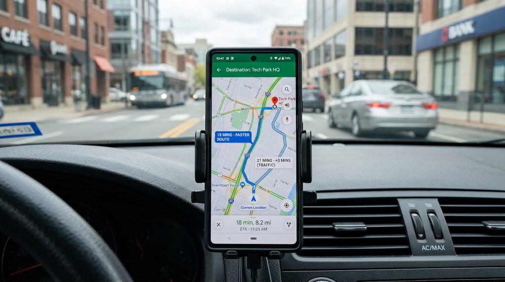
In many respects in modern technology, relationships between objects occur in transportation, communication, commerce and social interaction and make graph algorithms useful for a variety of areas. A GPS navigation system maps the vertices of roads and the vertices of intersections and maps the edges as the roads themselves. Route-planning systems can search for proper journeys by assigning weights depending upon distance, estimated travel time and other factors. The social network relies on graph structures, which represent users and their relationships, enabling applications to find common friends, recommend friends, and study communities.
Computer networks can be represented as graphs, where vertices represent computers and the links represent connections between them, allowing engineers to analyze the network and determine potential paths for data to flow. Delivery companies can be mapped as a connected node in the warehouse and/or distribution centre as well as the customer destinations, and graph algorithms can be used to analyse routes and optimise logistics plans. User graphs can be used to link users, products, interests, and activities to recommend products. These applications show that graph algorithms have uses beyond academia. They offer hands-on approaches to understanding complex networks, finding relationships and making decisions about the relationships between elements.
Challenges and Limitations of Graph Algorithms
Despite their usefulness, graph algorithms can present challenges when applied to large or changing networks. A graph containing millions of vertices and edges may require considerable processing time and memory, especially if it is densely connected. Selecting an unsuitable representation can make common operations unnecessarily expensive. Some algorithms also have specific requirements that must be satisfied for their results to be correct. Dijkstra’s algorithm, for example, assumes non-negative edge weights, while minimum spanning tree algorithms are generally applied to undirected weighted graphs.
Real-world networks may also change while a program is operating. Traffic conditions can alter travel-time estimates, communication links can fail, and users can establish or remove relationships on a social platform. Systems that work with dynamic graphs may need to update their analysis rather than recalculate every result from the beginning. In addition, graph models simplify reality: a road represented by an edge does not automatically capture every factor affecting a journey. Developers must choose meaningful weights, maintain accurate data, and account for relevant constraints to ensure that an algorithm’s results are useful.
Conclusion
Graph algorithms provide powerful methods for understanding and processing relationships between connected objects. By representing information as vertices and edges, computers can analyze networks that would otherwise be difficult to examine systematically. Breadth-first search explores connections level by level and finds paths with the fewest edges in unweighted graphs, while depth-first search investigates one branch at a time and supports tasks such as cycle detection and connectivity analysis. Dijkstra’s shortest-path algorithm calculates minimum-cost routes when edge weights are non-negative, and minimum spanning tree algorithms identify economical ways to connect all vertices in an undirected weighted network.
These techniques support applications ranging from GPS navigation and delivery planning to social networking, recommendation systems, and computer communications. However, successful implementation requires more than knowing how each algorithm works. Developers must understand the graph’s structure, choose an appropriate representation, consider computational complexity, and ensure that the algorithm’s assumptions match the problem. As digital systems continue to generate and depend on connected data, graph algorithms will remain important tools for discovering relationships, improving efficiency, and solving complex network problems.