
Introduction
The main reason why algorithms are considered essential to computer science is that they offer a methodical approach to tackling issues, manipulating data, and performing calculation tasks. An algorithm is a set of explicit instructions which explains how to obtain a given output. Algorithms are used in computers to work on common tasks like searching information, sorting data, suggesting products, driving roads and handling financial transactions. While some algorithms include only a few simple processes, others have complex operations that can manage millions of records, or deal with difficult mathematical problems. An algorithm’s properties aid software developers in creating efficient, reliable, and easier-to-maintain software. There are a variety of problems that call for different approaches, and computer scientists have created several ways of working with algorithmic strategies. Students who have knowledge about computer science algorithms will have the base of understanding of the efficient solution to computer problems.

What are Algorithms and Why are they Important?
Algorithms are a finite number of instructions that can be used to convert an input into a desired output or to perform a particular task. For instance, if you are making a cup of tea, that could be as simple as boiling water, putting a tea bag in a cup, pouring in the hot water and letting the tea steep. The principle is the same with computer algorithms, but the instructions are written in a language called a program, as a mathematical operation, or as logical rules. When an algorithm is written to solve a finite problem, it should stop after a finite number of steps; the algorithm has to be precise enough that these steps can be followed. Algorithms have been a major consideration in computer science since they decide the efficiency of software operation. Depending upon algorithms, two programs can achieve the same result, but give vastly different time and memory requirements.
Algorithms can also be used to divide up a difficult problem into smaller steps. Imagine an online bookstore with thousands of books to be organized by title, find a specific book and suggest other items to the shoppers. For each task, an appropriate algorithmic approach is needed and choosing an appropriate method can enhance the speed and reliability of the application. Time complexity and space complexity are frequently used to talk about the efficiency of an algorithm. The time complexity is the number of operations that increases with the increase of the input size and space complexity is the amount of extra memory that an algorithm uses. Programmers use big O notation, e.g. O(n), O(log n), O(n²), etc., to describe these growth patterns. Once developers have a grasp of these concepts they are able to evaluate the available solutions and select methods that will not become impractical due to the size of applications and data.
1. Sorting Algorithms
Sorting algorithms organize information based on a given order, such as ascending numerical order, descending numerical order, or alphabetical order. They are generally used in databases, spreadsheets, search mechanisms, e-commerce, and applications handling huge lists of records. For example, a website that offers online shopping could categorize the products by price so that customers can easily find the products that are the cheapest. Likewise, a school management system could have students’ records sorted alphabetically or exam results sorted by highest to lowest. Other operations may be easier if data is organized because it’s easier to search, compare, and analyze organized data. Each of the sorting algorithms has a strategy to accomplish a general goal and each of them is affected by the number of items, the order of the data collection in memory and the memory available.
This is the list of commonly used sorting algorithms.
Bubble Sort
Bubble Sort compares adjacent elements and swaps them around until they are in order. This process repeats as long as the elements are not in the correct order. For instance, if the numbers are 5, 2 and 4, then the sorting algorithm compares 5 to 2, swapping them if 5 is greater, and then compares 5 to 4, swapping them if 5 is greater.
The sequence is now 2, 4 and 5. Bubble Sort is a simple algorithm to understand and implement and can be helpful for introductory programming problems. Its average and worst case time complexity, however, is O(n²) and this makes it inefficient if the dataset is large.
Selection Sort
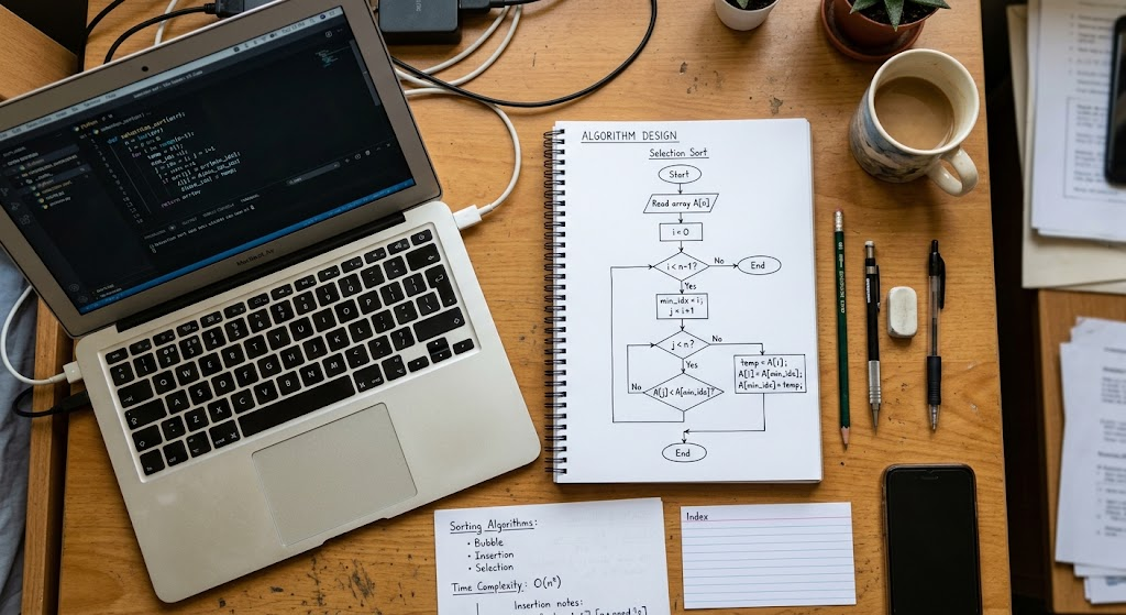
Selection Sort iterates through the unsorted portion of a collection and finds the smallest element of the unsorted portion and swaps it with the first element. When the input is 7,3, and 5, the algorithm will choose 3 and set it to the first position.
It then picks up 5 of the remaining elements, thus giving 3, 5, and 7. Selection Sort is simple and only makes a few swaps, and normally takes O(n²) comparisons. Thus, it is more appropriate for the design of learning algorithms or for small collections than for very large data sets.
Merge Sort
Merge Sort is an efficient approach to sorting data with the divide and conquer method. It splits a collection into smaller parts, sorts each part in isolation and then combines them to form a single sorted collection. For example, the sequence 8, 3, 6, 2 can be divided into two smaller sequences: 8, 3 and 6, 2.
The results are sorted in each section prior to summarizing in 2, 3, 6, 8. On average Merge Sort takes O(n log n) time and works well with large data sets. The major drawback is that many implementations will need extra additional memory to join.
Quick Sort
Quick Sort is a sorting algorithm that first picks an element in the data stream as pivot and then divides the data into two groups: those less than and those greater than the pivot. Then it recursively sorts the resulting sections. When sorting 6, 2, 9, 4, the algorithm could choose 6 as the pivot, move the smaller numbers to the left and the larger numbers to the right and then sort the smaller and larger parts.
Quick Sort worst case time is O(n²) but with an average time of O(n log n). It is generally studied due to the fact that it could be executed efficiently in a practical application, especially if executed with appropriate pivot-selection techniques.
2. Searching Algorithms
A search algorithm is used to find out a particular information in a data collection. They are vital for performing tasks like looking up customer records, searching for a product, searching for a file, searching for a database entry, or determining if there’s a specific value in the database. Suppose there is a school database that has thousands of student records. When the administrator enters the identification number of a student, a search algorithm is used to find the student’s record. The best search method will vary depending upon how the information is stored and organized. A few algorithms consider each element sequentially, others can determine the structure of the data set to discard significant parts of the search space. Choosing an efficient search algorithm can lower search times and enhance the users’ experience when users require information to be quick.
There are many types of searching algorithms.There are various types of searching algorithms.

Linear Search
Linear Search is a search technique that examines the elements sequentially, starting from the beginning and moving toward the end of the collection, stopping on a match or reaching the end. Suppose a list contains 12, 7, 19, 4, and 15, and the goal is to find 4.
The algorithm starts with the 12, then 7, then 19, and finds the 4. Linear Search is flexible and easy to implement, as it can be used on both sorted and unsorted data. The worst case time complexity is O(n) which means the number of checks can increase linearly with the number of elements. It may be appropriate in small collections, or when data is not in an appropriate order to use.
Binary Search
Binary Search searches for a target by recursively dividing the sorted collection into two parts. Compares the target to the middle element and figures out which half might have the target value. The algorithm, for instance, looks at the middle value in the sorted list 10, 20, 30, 40, 50; and, if the mid value is less than 30, then the algorithm narrows the search range to the lower half of the list, or if the mid value is more than 30, then the algorithm narrows the search range to the upper half of the list.
The advantage of Binary Search over the Linear Search is that its running time is O(log n) which is much faster than O(n) for large sorted collections. The data, however, needs to be sorted, and the implementation needs to enable easy access to the middle element for the usual performance benefit to be gained.
3. Recursive Algorithms
A recursive algorithm is an algorithm that is a function that calls itself with a “smaller” or “simpler” version of its original problem. This technique is well suited when a problem can be naturally stated in terms of smaller problems of the same problem type. A recursive algorithm typically has a base case that indicates when to end the algorithm, and a recursive case that breaks the problem down and then calls the algorithm again.
Recursion can loop endlessly or cause a “stack overflow” without a base case or a reliable means to return to the base case. Tree traversal, mathematical calculations, exploring a file system, and divide-and-conquer algorithms are among the common applications of recursion. This can help make some solutions more understandable, as the code doesn’t explicitly control each intermediate step, but rather reflects the structure of the problem.
Example of a Recursive Algorithm
One of the classic examples is computing the factorial of an integer. The factorial of a positive integer n is the product of all positive integers from n down to 1. For example, 4! equals 4 × 3 × 2 × 1, which produces 24. A recursive definition is one in which a thing is defined in terms of one or more other things that have already been defined. n! = n × (n − 1)! where 0! = 1. Thus, a recursive function will recursively compute the factorial of a given number by recursively calling itself with increasingly smaller numbers until it reaches zero.
Then the results are returned via the series of calls. While recursion is elegant to solve this problem, it may not be the most efficient way to solve it for all problems. If recursive calls are going to store the states of the function calls, then an iterative version might be better to avoid “too many” calls to the stack or if there is unnecessary overhead.
4. Greedy Algorithms
An optimization problem can be solved by a greedy algorithm which chooses at each step what might seem to be the optimal choice. The algorithm does not consider all possible combinations of decisions, but takes a step locally that is optimal, and proceeds towards an overall solution. This strategy can be efficient as it may narrow down the number of possibilities that will be taken into consideration. Greedy methods are effective for some scheduling problems and for minimum spanning tree problems, and for optimization problems in which the selection rules are carefully defined.
A locally optimal decision may not lead to a globally optimal decision, however. If the greedy strategy is used, developers need to make sure that it is suitable for the given problem. Under certain mathematical conditions, a greedy algorithm can yield satisfactory solutions and have a relatively low computation cost.
Example on How to Implement the Greedy Algorithm.
Suppose a delivery company must tie together a number of places by a road network, but wants to spend as little as possible on the roads. This is a greedy algorithm to find the MST of a connected, weighted graph. It looks at the edges available in order of weight, and picks out an edge if it does not form a cycle. For instance, if there are three locations: you can go between them with roads of cost 4, 6 and 9, then the algorithm would use the roads that cost the least, but not introduce unnecessary cycles.
The procedure is repeated until all locations are connected. The algorithm of Kruskal generates a minimum spanning tree of a graph under certain conditions. In this example, the problem of optimizing a complex network is solved by using a carefully designed greedy rule that avoids an examination of all possible networks.
5. Divide-and-Conquer Algorithms
Divide and conquer algorithms is a technique that breaks a problem into smaller subproblems, solves each of the subproblems and then combines the results. The typical steps used in the method are those of divide, conquer and combine. When dividing the problem is broken up into smaller pieces. In the conquering stage each part is solved, usually recursively.
Finally, the results are put together in a solution to the original problem. This technique works particularly well for problems that can be broken down into smaller subproblems, where each subproblem can be solved separately and efficiently combined. Sorting, numerical computation, image processing and large problem decomposition are examples of applications of divide-and-conquer algorithms.
Example of Divide-and-Conquer
Divide and conquer is another example of a well-known algorithm: Merge Sort.Merge Sort is one of the well-known divide and conquer algorithms. The binary search is an example of such a method – it always halves a sorted collection. However, these algorithms operate slightly differently: Merge Sort will take sorted subcollections and merge them together, binary search can eliminate half of the remaining subcollection of the search space after every comparison.
One way that divide-and-conquer methods can help is that they may break up a large computation into multiple smaller computations. Merge Sort, for example, has a complexity of O(n log n); in general, this is more efficient for larger data sets than straight quadratic sorts. However, this method isn’t always applicable. Some problems have subproblems that cannot be solved independently of each other or they require taking a long time to solve, and the benefits of dividing the computation are diminished.
6. Backtracking Algorithms
Backtracking algorithms follow the process of building a candidate solution of a problem incrementally. If the algorithm finds that a partial candidate cannot be extended to a correct answer, it backtracks over the last move in search of a different partial answer. This is repeated until a satisfactory solution is achieved or until the feasible solutions are explored. Backtracking is especially helpful for constraint satisfaction problems, puzzles, multi-way combinatorial searches and problems involving multiple decisions that have to meet multiple rules.
A backtracking algorithm can prune bad partial solutions at an early stage, rather than filling in all possible candidates. For many cases backtracking is more useful than the exhaustive enumeration method, because it can prune away unpromising solutions, but its worst case run time can be exponential in the number of possibilities.
Example of a Backtracking Algorithm
The N-Queens problem is an example of a backtracking problem. The objective is to position a given number of queens on a chessboard such that no two queens are attacked by more than one other queen. Each placement will have to meet a number of rules as queens can attack in rows, columns, and diagonals. A backtracking algorithm will place a queen in a valid position, go up a row and try again. If a placement leads to a conflict, then the algorithm removes the previously placed queen and tries another placement.
This is repeated until all the queens have been placed or until all possible arrangements are tried. These same methods can be used to solve Sudoku puzzles, to find combinations, and to find paths through mazes. Backtracking can be useful when the problem is such that a systematic approach is necessary, but can also be used to give rules to discard some of the choices before the whole solution is built.
7. Dynamic Programming Algorithms
Dynamic programming is an algorithmic methodology used for solving a problem that is broken up into subproblems, whose results are stored and then used for the solution of the larger problem. It is often helpful when the same subproblems are repeated many times and the problem in question can be formulated in terms of relationships between smaller subproblems. A recursive algorithm could calculate the same result multiple times, using up processing time; dynamic programming avoids that. Dynamic programming tries to solve this problem by storing previously computed solutions.
There are two popular methods for implementing it: one is to store values as they are computed by a recursive algorithm and the other is to accumulate a table of solutions to smaller problems and use it to solve more complex ones. Dynamic programming may need more memory, but when there are many subproblems to repeat that are an expensive part of the computation, then it can significantly enhance the speed of the algorithm.
Example of a Dynamic Programming Algorithm
Dynamic programming is an easy example that is provided by the Fibonacci sequence. Here the numbers after the first two are the sum of the two numbers before them. Starting with 0 and 1, the sequence continues as 0, 1, 1, 2, 3, 5, 8, and 13. The basic recursive solution recalculates the previous Fibonacci numbers repeatedly, which causes a significant amount of duplication when the input size increases. By using dynamic programming, the process can be improved by storing each value computed and using it later on demand.
The algorithm starts from the first two values and calculates the remaining values in order, starting with a “bottom-up” approach. The naive recursive solution takes exponential time to calculate the first n Fibonacci numbers, while the above solution only takes linear time. Dynamic programming is also used in problems such as resource allocation, optimal combinations under certain conditions, scheduling, and comparing texts.
8. Brute-Force Algorithms
In a brute force algorithm, one simply tries out all possibilities without using a more sophisticated shortcut. The technique is simple and straightforward, as it essentially goes with the requirement of the problem. For instance, a brute force search could check each element of a collection to see if a certain value is in the collection or not. Likewise, there might be a small puzzle to be solved by trying all blocks of possible arrangements until a right answer is found.
Brute force is helpful when the problem is small, when a simple solution is desired, or when it serves as a reference solution to test the more complex solution. But the number of possible candidates can escalate quickly with the increase in the input. Brute force techniques are therefore often not useful for large optimization problems, though they are useful in algorithm design, correctness testing, and where the search space is small.
Example of a Brute Force Algorithm
Suppose there is a program which has to find two numbers in a list which add up to a value. Brute Force: Iterates through all possible pairs, checking if they satisfy the condition. Now, if the list is 2, 7, 11, 15 and the target number is 9, then the algorithm will eventually find 2 and 7. If this is the case, then it will take O(n²) time to check each pair since each element would have to be compared to many other elements. Row 2.26 shows an alternative solution with a hash table that can solve the same problem in expected O(n) time by storing the previously encountered values and checking if the value to find is the complement of the stored ones.
The example shows why brute force can be a good starting point, but not necessarily the ultimate solution. Just starting with a simple approach can help developers grasp the problem first and then make optimizations.
How to Select the Appropriate Algorithm
Choosing an algorithm involves knowing about the problem, its input and its available resources. Linear Search could be effectively used for searching elements in a small unsorted collection and Binary Search could be used for searching elements in a collection with elements arranged in sorted manner. Likewise, Merge Sort or Quick Sort can be used for larger sets of data; however, a simple sorting algorithm can be used for a smaller set of data for an introductory exercise. Some repeated-subproblems problems can be solved with dynamic programming, and others have constraints and are more suitable for solving with backtracking. Memory requirements, the complexity of implementation, reliability and whether or not the algorithm provides an optimal result, are also important considerations for the developers. An algorithm which is efficient for a small test data set may become inefficient on larger inputs – realistic workloads and growth must be taken into account when evaluating.
Although it can be a good reference point to compare the efficiency of algorithms, it should not be the only one to consider when making the decision. On the other hand, an algorithm that has a better theoretical complexity could have implementation overhead that will result in the other algorithm being faster for small input sizes. Similarly, if an application is being run on a device with limited resources, a method that consumes less memory than another could be desired. When programming, the worst case, average performance, data structure and the implications of poor results should be all taken into account. Testing and benchmarking can show performance in typical use scenarios. In production software, the best algorithm will usually be the one that satisfies the correctness and performance needs of the application, is maintainable, and is implementable.
Examples of Real-world Applications of Algorithms.
A lot of the digital services users use every day are supported by algorithms. To find relevant information from vast collections of documents, search engines use ranking and retrieval algorithms. Graph algorithms and optimization techniques are used in navigation applications to find routes based on distance, estimated travel time, and road conditions. Algorithms are crucial for online stores for product sorting, inventory management, item recommendation, and transactions. Computational techniques are employed by financial platforms to verify business activities, review records, and identify any suspicious activity. In healthcare, algorithms can help to sort patient data, analyze medical images, or assist in data analysis. The algorithm should be suitable for each task and the data it manipulates in each case. When the outcomes have an impact on financial decisions, safety or access to critical services, correctness, reliability, and efficiency are of special importance.
In addition to its role in image processing, algorithms have many other important applications in AI, machine learning, cybersecurity, and scientific research. Optimization algorithms are used in machine learning systems to tune the model parameters during the learning process, and graph algorithms are used to analyze the relationships in social networks and communication systems. Certain sequence-comparison and resource-allocation problems can be aided by dynamic programming; and some problems with complex constraints can be solved with backtracking. These applications show how algorithms are not just academic theories; they’re real tools for software systems to work with data to get useful results. With the increasing size of data sets and the complexity of computing environments, the developers’ challenge is ongoing, requiring them to assess and refine algorithmic decisions to guarantee responsiveness, scalability, and reliability in their systems.
Conclusion
Algorithms are crucial in computer science, as they are used to solve computational problems in a structured way. Sorting algorithms arrange information, searching algorithms find information and recursive algorithms represent solutions in terms of smaller versions of the problem. A greedy algorithm works by making locally optimal decisions and a divide-and-conquer algorithm breaks down a large problem into smaller problems. The Backtracking algorithm is used to find all possible solutions, but not to choose solutions that are invalid, and dynamic programming uses memoization to store and re-use the results.
Brute force algorithms provide simple solutions which can be useful for small problems and as references for optimisation. Both have pros and cons and will work best in particular circumstances. Knowing these differences can guide programmers to choose appropriate strategies, minimize redundant calculations, optimize memory usage, and create robust programs. Understanding algorithms is crucial for any aspiring programmer, especially beginners, to master the art of problem-solving and develop a solid grasp of computer science.