Introduction
Discrete mathematics is a field concerned with countable structures, such as integers, sets, logical statements, graphs, relations, and sequences, etc. Continuous mathematics deals with continuous quantities, whereas in discrete mathematics, the objects are those that can be divided into discrete parts. This is important in computer science as a computer processes information and performs discrete operations like evaluating conditions, comparing values, storing data and executing instructions. These mathematical principles are key to the algorithms that are used to solve computational problems step-by-step. Discrete mathematical ideas are the tools that can be used to reason about a problem and to solve it, whether a programmer is writing a sorting program, designing a search engine, studying a computer network, or designing a database system. Knowing these ideas enables programmers to write better code than seems to work, into programs that are logically sound, demonstrably correct, and computationally efficient.
When looking at the different phases in the development of an algorithm, the connection between discrete mathematics and algorithms is especially apparent. Programmers need to know the problem, what its inputs and outputs are, the possible cases and what method they need to use to solve the problem before implementing a solution. The techniques of discrete mathematics are used to help in each of these stages: Representing information, analyzing relationships, proving correct, and estimating performance. For instance, Logic can be used to build reliable conditional statements, Graphs can be used to determine routes and analyze networks, and Combinatorics can approximate the number of possible arrangements or solutions. A mathematical proof can be used to show that an algorithm always gives the correct output for all correct inputs, and asymptotic analysis can be used to describe the behaviour of its running time as the input size increases. These concepts will be illustrated through examples of programming problems, helping students understand the importance of algorithms and how to optimize them.
Algorithms and Their Mathematical Foundations
An algorithm is a sequence of instructions that is a finite sequence of well-defined instructions for solving a problem or completing a computational task. They are used in tasks such as identifying the maximum value from a list of values, looking for a specific record among a set of records, sorting a list of names by alphabet, and finding the shortest path between two points in space. Though they may look distinct, they all have one thing in common – they all require a systematic process that takes an input and outputs the desired output. Programmers use discrete mathematics to precisely describe these procedures, and to investigate what happens to them when they are faced with various conditions. For example, an algorithm which determines the greatest element of a list needs to consider all the elements, even negative ones, the repeated elements, and lists of only one element. By using mathematical reasoning, the programmer can make the assumptions of the algorithm, specify the condition that the algorithm is valid and decide whether the algorithm gives the right answer.
Suppose a function exists that is supposed to return the largest element of an array of numbers. The algorithm starts off by setting the first element as the current maximum, then compares each of the elements after that with the current maximum, and updates the maximum if it finds a greater value. It will return the largest element of the array after the processing. This is a simple procedure, but with some reasons explained mathematically. Each element should be checked on a by one basis, and the current maximum value should be the greatest value among all values processed until now. This property is called an invariant and serves as a basis to prove that the algorithm is correct. The algorithm also demonstrates how an expression composed of simple mathematical operations can capture a convenient computational attribute. Knowing what the invariants are, a programmer can think about more complicated algorithms such as sorting procedures, search algorithms, and iterative calculations, without simply taking a look at the code or testing it.
Mathematical Induction and Algorithm Correctness
Mathematical induction is a method of proof that is applied to prove a statement for all integers within a given set, typically all integers n ≥ n0. Many algorithms have inputs that grow larger and larger or execute repetitive tasks, which makes it particularly useful in computer science. The technique consists of two important steps: the base case, and the inductive step. If one doesn’t write anything, the statement is true for the initial value. The inductive step in the proof is to assume a statement is true for any given value and show that if this happens, then the statement is true for the next value. These stages form the proof that the statement is true for every number in the sequence. For a more detailed explanation about the technique, read the book on mathematical induction. Induction is often applied in the development of algorithms to establish properties of recursive algorithms, iterative processes, and mathematical formulas that model the behavior of algorithms.
A simple example is to show that an algorithm is correct when it adds up the first nn positive integers. The mathematical formula for this sum is 1+2+⋯+n=n(n+1)21+2+\cdots+n=\frac{n(n+1)}{2}. Start the induction proof at n=1n=1. The sum is 11, and the formula gives 1(1+1)2=1\frac{1(1+1)}{2}=1, so the statement holds. Next suppose that the formula holds true for any positive whole number nn. Existing sum plus n+1n+1 is therefore the sum of the first n+1n+1 integers, or n(n+1)2+(n+1)\frac{n(n+1)}{2}+(n+1). If we simplify this expression we get (n+1)(n+2)2\frac{(n+1)(n+2)}{2} which is precisely the formula that we want for n+1n+1. This proof is used to show an extension of an existing proof to a larger input. A similar approach can be used to define correctness properties for recursive algorithms and to ensure that the programmer realizes that successive execution steps will keep the desired result.
Mathematical Proof Techniques Used in Algorithm Design
Mathematical proofs are the tools of the trade for proving statements to be true under given conditions. In computer science, they are used to prove that an algorithm is correct and meets the required conditions, as well as consistently producing the desired results for all valid inputs. There are some proof techniques that are especially useful, such as direct proof, proof using contradiction, proof by contrapositive, and mathematical induction. In a direct proof, the assumptions are known, and then these facts are used to logically show the desired result. Proof by contradiction assumes the negation of the conclusion and shows that this assumption would result in an inconsistency. The proof by contrapositive is one way to prove an implication by proving its logically equivalent contrapositive. The techniques are each different ways of solving hard reasoning problems and using a suitable technique can make an argument clearer. The techniques are useful as an algorithm can fail a number of tests, yet still not be correct for all possible inputs.
Describe binary search, which is an algorithm that locates a value in a sorted array by always testing its middle value and discarding either the first half or the second half of the array as needed. It can be proven to be correct with an invariant which reads if the number x exists in the array it is still in the current search interval. At the start, the interval contains all of the array, thus the invariant is satisfied. If the middle term is the target, then the algorithm has the answer. Since the smaller element is guaranteed to be to the left of the middle element, when the target is smaller than the middle element, then it cannot appear to the right of the middle element. If the target is bigger it cannot be to the left. So the algorithm can safely delete the irrelevant half, without losing the possibility of locating the target. Eventually, the interval will be empty or there will be a target found. This argument is correct as long as the input is sorted and interval boundaries are taken into account during implementation. Formal proofs can aid developers in discovering vital assumptions and also subtle implementation mistakes.
Mathematical Logic and Conditional Reasoning
In mathematical logic, one focuses on statements, truth values, logical operators and the links between propositions. The concept of a condition is basic to programming, since algorithms rely on conditions to decide which instructions to take. Logical operators such as AND, OR, and NOT are equivalent to conjunction, disjunction and negation. An AND expression will return true if both of the conditions on the AND are true, an OR expression will return true if either of the conditions on the OR is true. NOT flips the truth value of a statement. These operators are used by programmers in conditions, loops, validation rules, access controls and search filters. Their mathematical significance can assist developers to build expressions that perform as desired. It also often makes it easier to find logical errors such as wrong combinations of conditions, wrong parentheses or guessing whether a statement is true or false at some point.
For instance, a service provided online could only be used by a user if they had an active account and the necessary permissions to use it. This rule can be written as A∧PA \land P, where AA is the active account and PP is the permission of the user. Access will only be given if both are true. In a different rule, the access might be granted if the user is an administrator or they are given a special permission, denoted by D∨PD \lor P, with DD representing the administrator status. The examples below show how policy requirements are mapped to exact computational conditions by means of logical expressions. Loops and the termination of algorithms can also be reasoned about using logic. A loop condition tells whether the loop will be repeated or not repeated; a loop invariant is a property such that it is always true when the loop is repeated. Programmers can develop algorithms which can consistently process different inputs and minimize unexpected behavior by carefully reading these statements.
Sets and Their Applications in Algorithms
Set theory is the study of sets and their relationships. Numbers, names, database records, and other elements that are well defined can all be included in a set. Some important operations are union, intersection, difference, and membership testing. The union of two sets consists of all elements that are in either set while the intersection consists of all elements which are in both sets. The set difference finds elements that are in one set but not in the other. These operations are directly applicable in the computer science world, such as in database queries, search systems, recommendation systems, and data filtering. A common use of sets is to represent sets of objects and find out what objects are contained in each set and how they overlap. Set theory is also very useful for the design of algorithms that eliminate duplicates, find common elements or determine if items have already been processed.
Suppose there is a system with 2 sets of users: one for users who registered for a programming course, and one for users who registered for a mathematics course. Intersection shows the users who have been enrolled in both courses, and union shows the users who have been enrolled in either of the two courses. The difference between the two sets (programming-course set minus mathematics-course set) is users who registered for programming but not mathematics. These operations can be used to enable enrollment reporting, personalized recommendations and administrative choices. Sets also are used in graph algorithms, where the programmer keeps lists of “visited” vertices, “unprocessed” vertices, or “candidate” solutions. For instance, in a graph traversal, it can keep a set of all visited vertices, to prevent traversing the same vertex multiple times. If, for a particular data structure, membership testing is efficient, this can spare unwanted work and ensure that the algorithm works correctly on graphs with cycles.
Relations and Their Role in Data Organization
A relation is a relationship between elements from one set and the elements from another set or with other elements from the same set. Relations can be shown as sets of ordered pairs, for example {(a,b), (a,b)}, which indicates that there is an association between aa and bb. Relations have significance in computer science as a model for database relationships, dependency structures, ordering rules, and network relationships. Certain relationships have mathematical characteristics such as reflexive, symmetric, antisymmetric and transitive. A relation is reflexive if every element in it is related to itself, symmetric if the relation between two elements in the relation implies a relation between the other two, and transitive if every element in it is related to the last element in the relation. Knowing these properties facilitates the programmer to select a suitable representation and reason about the behavior of an algorithm that acts on connected information.
For instance, a relation of employees and departments in a database could be a relationship between employees and their working departments. There can be a separate relation between employees and their supervisors. These relationships enable the system to respond to queries on the structure of the organization, its reporting requirements, and its departmental members. Relations can also be used for dependency analysis with software development. An ordered pair can be used to represent a dependency if one task must be done before another task. A set of these dependencies can then be analyzed to find a valid order to execute. If there are no cycles in the dependency graph, it is possible to use a topological sorting algorithm to create an ordering that satisfies all requirements. Using relations to precisely capture connections allows programmers to create algorithms to solve scheduling problems, to organize data in a database, and to analyze complex systems without depending on a general description of the way in which individual objects are related.
Graph Theory and Network Algorithms

Graph theory is the study of structures made up of vertices, or nodes, and edges, which link two vertices. Graphs can be used to represent relationships in which the relationships are important, not the objects themselves. For instance, a road network can be represented as a graph, with intersections at nodes and roads as links. People can be represented as vertices and relationships as edges of a social network. Graphs can also be used to model computer networks, transportation systems, recommendation engines, and links on websites. Graphs can be directed, undirected, weighted or unweighted, depending on the problem. Directed edges are those where the relationship is one way, undirected edges are those where the relationship is not specified. Weighted edges have extra attributes like distance, travel time, or cost. The differences enable graph models to be used to represent many real-life problems, and to give mathematical form for specific algorithms.
There are several key algorithms that are applied to graph structures. BFS traverses a graph level by level and can be used to find a shortest path (in an unweighted graph). DFS works by diving deeply into one branch, and then back up to the previous branches. It is helpful when trying to solve connectivity problems, cycle detection problems, and similar tasks. Dijkstra’s algorithm works on the problem of finding shortest paths from a starting vertex in a graph with non-negative edge weights. Suppose that we have a navigation app that needs to find a path between two points that is as efficient as possible. The application may be used to model intersections as vertices and roads as weighted edges, where weights are the distance of the road or the expected time of travel. A shortest-path algorithm next looks at the possible routes and one with the lowest total weight is chosen. The success of such a solution depends on the ability to choose the proper graph representation and algorithm for the problem’s limitations. Graph theory thus shows how such abstract mathematical objects can be used practically to solve routing, scheduling and network analysis problems.
Combinatorics and Counting Computational Possibilities
Combinatorics is a branch of mathematics that deals with the number of arrangements, selections, and possible outcomes. It’s also useful in algorithm design, as the programmer may want to see how many possibilities there are in the problem to decide upon a method of solution. Examples of commonly used tools in the combinatorial world: product rule, sum rule, permutations, and combinations. The product rule is that if a process involves a sequence of independent choices, each of which has a known number of possible choices, then the number of possible outcomes is equal to the product of the numbers of choices for each of the independent choices. The sum rule is used to add together the numbers of alternatives that are mutually exclusive. Permutations give the number of ordered arrangements, combinations give the number of unordered selections. The following principles are useful for programmers to analyze a search space, evaluate an exhaustive algorithm, design test cases, and understand why one might need to seek a solution to a computational problem, and why it can be costly as the size of the problem’s input increases.
Let’s say that an algorithm checks all the possible permutations of nn distinct objects. There are n!n! different ways to arrange them, where n! is defined as n!…n(n-1)(n-2)\cdots 1 If the number of objects is moderately increased, the number of arrangements can be very large. For instance, five distinct objects have 5!=1205!=120 possible orderings, while ten have 10!=3,628,80010!=3,628,800. As the problem becomes increasingly complex, an algorithm that checks all arrangements might become impractical. The traveling salesperson problem is an example of this type of problem, in which an optimum tour might require looking at many routes through a group of cities. Combinatorial reasoning provides insights into the scope of the search space and is used to provide motivation for pruning, backtracking, dynamic programming, and approximation algorithms. Programmers can use the pre-implementation estimation of the number of possibilities to make better decisions about the selection of the algorithm and the requirements for resources.
Recurrence Relations and Recursive Algorithms
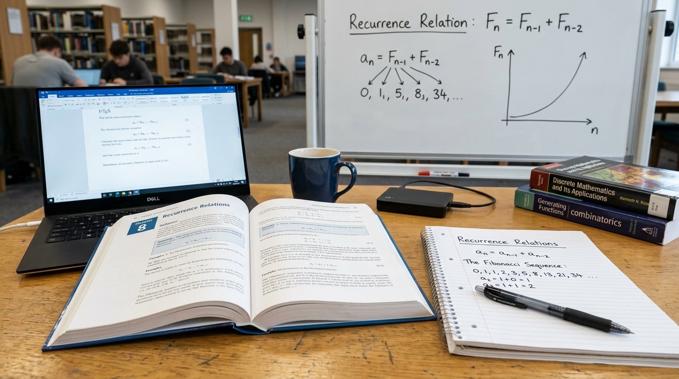
A recurrence relation is a way to define a mathematical sequence by using one or more previous terms. Recurrence relations are frequently used in algorithm analysis to represent the running time of recursive algorithms. A recursive algorithm works by breaking down a problem into smaller and smaller problems of the same type until it reaches a base case where it can be solved. Thus the total computational work is determined by the work done by the recursive calls as well as the work done on each separate call. A recurrence can be used to symbolically describe this relationship mathematically. For instance, an algorithm could split an input into smaller pieces, solve each piece recursively, and then merge the solutions. If it takes more time, it can often be expressed with a recurrence that involves the size of the subproblems, and the extra work needed to bring the subproblem solutions together.
Merge sort is an example. This sorting algorithm works by partitioning an array into two nearly equal-sized subarrays, sorting the subarrays, and then combining them together. With nn elements in the input, each of the two recursive calls will process about nn/2n/2 elements, and the linear time required to merge the two sublists is the number of elements that got divided. Thus, the recurrence is T(n) = 2T(n/2) + O(n)T(n) = 2T(n/2) + O(n) with a constant-time base case for values of n below some threshold. If the recurrence is solved, it will be O(n\log n)O(n\ log n). This is the reason a simple quadratic sorting algorithm isn’t very good on large arrays compared to merge sort. Recurrence relations enable a programmer to compare recursive strategies, find costly operations, and to forecast performance as the input size increases. They are particularly useful when the algorithm is a complex operation in which you cannot understand the behavior from a single operation.
Asymptotic Analysis and Algorithm Efficiency
Asymptotic Analysis is used to study the growth behavior of an algorithm’s resource requirements as the size of its input grows. It does not calculate the exact execution time using one computer but it investigates the general trend of running time or memory consumption. This is helpful because real life performance is dependent on hardware, programming languages, compilers, etc. Many of these factors can be ignored by comparing algorithms using asymptotic notation. The upper bound of an algorithm is called Big O and the lower bound is called Big Omega. A tight asymptotic bound is called Big Theta if it is bounded above and below by constant multiples of the same growth function. Common complexity classes include O(1)O(1), O(logn)O(\log n), O(n)O(n), O(nlogn)O(n\log n), O(n2)O(n^2), and O(2n)O(2^n). Knowing these classes is important for programmers to assess if an algorithm is likely to be practical for larger problems.
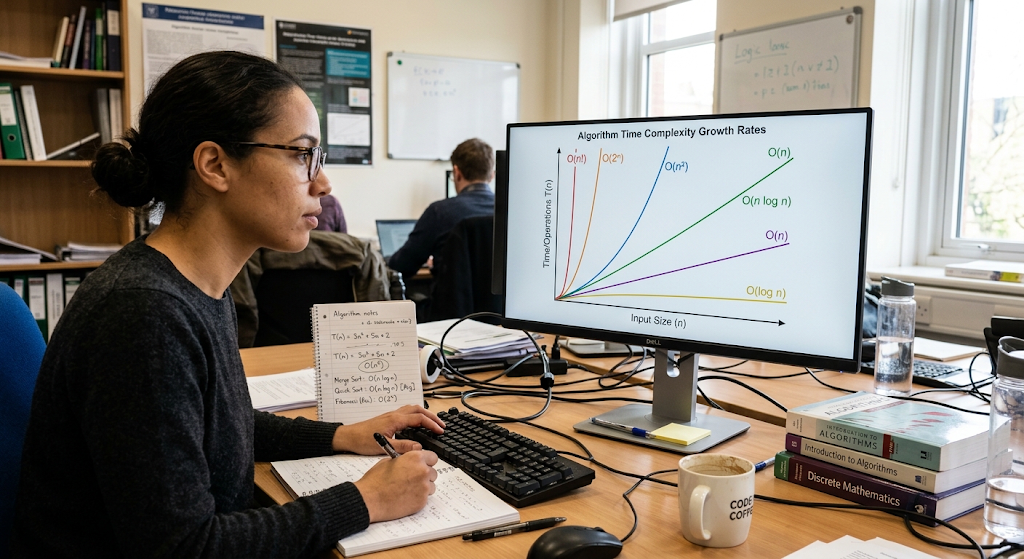
Suppose that you have two algorithms to find an element in a sorted array. Linear search looks at them in sequence and could require checking all nn elements, so the worst case time complexity of linear search is O(n)O(n). There is a repeated halving of the search interval in binary search, making the worst case time bound O(logn)O(\log n). The difference is negligible for a small array, but significant for large ones. In the worst case, the linear search on an array of ~1 million elements will need ~1 million comparisons, whereas the binary search will need only ~20 comparisons. This comparison assumes that the array is sorted and that the search code is correct. If sorting is necessary, it should be done first, and the cost of the sorting should be taken into account when considering the entire solution. Therefore, asymptotic analysis can be helpful for a developer to compare the approaches fairly, to realize the scalability limitation and to select the algorithm for the workload that they anticipate.
Combining Discrete Mathematics to Solve Complex Problems
Each of these different aspects of discrete mathematics provides specific tools, but in the real world, the development of an algorithm may involve a combination of these concepts. There are many examples in different domains that can utilize sets. For a programmer solving a scheduling problem, sets can represent available resources, relations describe dependencies, graph theory is used to model connections, combinatorics can be used to estimate possible schedules, and asymptotic analysis can be used to evaluate competing algorithms. Scheduling constraints can be mathematically stated, and induction could be used to prove that a recursive procedure yields valid results. The running time of a divide-and-conquer strategy can be described using recurrence relations, and proof techniques can be used to prove that an optimization is correct. The ideas given together give a fuller method of computational problem solving than the treatment of each mathematical concept as a separate entity. It also nudges the programmer to choose the model and method appropriate to the problem structure, not just the more common coding patterns.
Suppose that a university system has to schedule exams into rooms and times, such that no student is given more than one exam at a time that overlaps with another student’s exam. A graph could be used to represent the problem where the vertices are the examinations and the connections between two examinations are represented by an edge if the two examinations cannot both happen at the same time because they share students. The problem now reduces to coloring the vertices with colors (or time slots) such that adjacent vertices are colored differently. This is an example of graph coloring. Combinatorics is used to estimate possible assignments and logical constraints are used to define which assignments are valid assignments. An algorithm can try out alternative programs and eliminate ones that fail to meet the requirements, and then look for a feasible program. The final assignment can be proven mathematically to satisfy the indicated constraints, and complexity analysis can be used to determine the behavior of the method with increasing numbers of examinations. This example demonstrates the use of discrete mathematics in the modelling, solving, verification and evaluation of a practical computational problem.
Common Challenges When Applying Discrete Mathematics to Algorithms
Learning to apply discrete mathematics in programming can be challenging because mathematical definitions often appear more abstract than ordinary coding instructions. Students may understand how to write a loop but struggle to express the property that makes the loop correct. Others may recognize a graph or recurrence relation in theory but find it difficult to identify the appropriate representation in a practical problem. These difficulties can be reduced by connecting each mathematical concept to a concrete example and explaining the assumptions behind the model. For instance, when studying binary search, students should understand why the input must be sorted, how the search interval changes, and why each discarded portion cannot contain the target. When studying graph algorithms, they should distinguish between directed and undirected edges and understand whether edge weights represent distances, costs, or another quantity. Such connections help transform abstract definitions into useful problem-solving tools.
Another common challenge is confusing an algorithm that works on a few examples with one that is correct for all valid inputs. Testing is important because it helps uncover implementation errors, but a collection of successful tests cannot generally prove universal correctness. Mathematical proofs address this limitation by establishing why the algorithm works under its stated assumptions. Students may also confuse theoretical complexity with actual execution speed. An algorithm with a better asymptotic bound may still perform worse on very small inputs because of implementation overhead or other practical factors. Therefore, algorithm evaluation should combine mathematical analysis with appropriate testing and consideration of the intended environment. By practicing proof techniques, examining edge cases, analyzing input growth, and implementing algorithms, learners can develop a balanced understanding of both the theoretical foundations and practical realities of computer science.
Conclusion
Discrete mathematics provides the foundation for designing, analyzing, and verifying algorithms because it offers precise ways to represent computational problems and reason about their solutions. Mathematical induction and other proof techniques help establish correctness, while logic supports conditional decisions and rigorous reasoning about program behavior. Sets and relations organize information, graph theory models connected systems, and combinatorics helps estimate the number of possible outcomes. Recurrence relations describe the behavior of recursive algorithms, while asymptotic analysis explains how computational requirements change as input sizes increase. These concepts work together to help programmers move from informal ideas to structured solutions that can be evaluated and justified. Rather than serving only as academic exercises, they provide practical tools for building reliable software and understanding why particular algorithmic approaches succeed or fail.
For students and aspiring programmers, learning discrete mathematics is an investment in long-term problem-solving ability. Programming languages and software frameworks may change, but the underlying principles of logic, proof, counting, graph structures, and algorithm analysis remain relevant across many areas of computing. Developers who understand these principles can identify hidden assumptions, compare alternative solutions, recognize performance bottlenecks, and explain why their implementations produce the expected results. They are also better equipped to study advanced topics such as artificial intelligence, cryptography, database systems, network optimization, and theoretical computer science. The most effective way to develop these skills is to combine mathematical study with practical exercises: formulate a problem, select an appropriate mathematical model, design an algorithm, prove its important properties, implement it, and evaluate its performance. Through this process, discrete mathematics becomes more than a collection of formulas; it becomes a systematic approach to solving computational problems correctly and efficiently.