
Introduction
Algorithms are fundamental to computer programming as a set of steps to solve a problem or carry out calculations. Computers are used in many programs to do the same thing over and over again, to process sets of data, or to divide up complex problems into smaller, more manageable ones. There are two popular ways to achieve these goals: recursion and iteration. Even though both are capable of tackling the same problems, they have different structures, processes, requirements for memory usage, and applicability in real life situations.
In programming, it is important to know these differences to select suitable methods in the development of efficient and reliable software. Examples of recursive vs. iterative include computing a factorial, looking for a value in a list, computing a Fibonacci Sequence, and traversing a tree structure. Both methods have pros and cons, so it is vital to understand the working before choosing the method.
What Is Recursion in Algorithms?
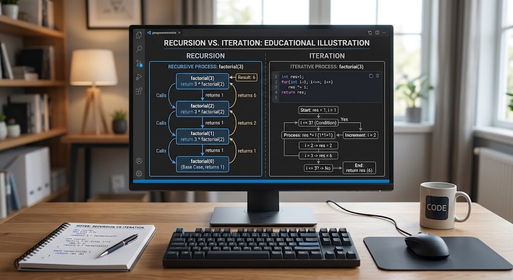
A programming method where a function calls itself to solve a problem by processing smaller problems of the original problem. In a recursive algorithm, a problem is reduced to a simple condition rather than repeated instructions being used to describe all the operations. However, if that is the case, it is called the base case and it will prevent any additional recursive calls from being made. Each call that is reducing the problem is part of the recursive case.
It is, for instance, the case for the factorial of a positive integer, which is equal to that integer times the factorial of the previous integer. The process is repeated until a calculation result becomes zero or some other end condition is reached. Recursion is especially valuable when a problem can be broken down into smaller, similar problems, like sorting files in a directory, handling hierarchical information, or solving some mathematical problems.
How Do Recursive Algorithms Work?
The recursive algorithm typically has three key elements: The recursive case, the function definition, and the base case. The function definition gives the operation the function performs, the recursive case will give the definition of the function called with a smaller or simpler argument. The base case is the case when the function does not return a result and does not call itself. A recursive function will have the result calls waiting until the result of their call is computed and while they wait, the result calls may be waiting for the result of another result call.
The call stack is a section of memory in which information about the current execution of functions is stored, and is used to manage these calls. When the base case is returned, the results are passed back up the function calls until the original operation is performed. It is important to understand this process as it can make a function call itself endlessly until it runs out of available stack memory if there is no base case or if the base case is incorrectly designed.
Example of Recursion: Factorial
A factorial is a mathematical function which is the product of every integer less than its argument. It is represented by an exclamation mark, for example 5! means 5 × 4 × 3 × 2 × 1, and the answer is 120. This number can be computed using a recursive algorithm: The factorial of the number n is defined as the product of n and the factorial of (n-1). In the base case, the factorial of 0 is defined as 1, so the calculations can be terminated. For example, factorial(5) calls factorial(4) which calls factorial(3), etc. until it reaches factorial(0) which returns the number 1. The waiting calls then multiply the numbers returned by each call by the numbers that each call multiplied by the waiting calls. This example shows how recursion can help to reduce the mathematical definition to the programming function, but also has some execution overhead per call, and uses memory to keep track of its state.
def factorial(n):
if n < 0:
Raising ValueError(“Factorial is not defined for negative integers”)
if n == 0:
return 1
return n * factorial(n – 1)
print(factorial(5)) # Output: 120
In this case, n == 0 is the base case and factorial(n – 1) is the recursive call. The function will keep decreasing the input till it reaches zero, after which the remaining calculations will return them. In this simple recursive solution, the number of function calls is in direct proportion to the number n and the amount of call-stack space used is O(n). Easy to understand, but not as good for very large inputs as recursion has a limited depth depending on the programming language and runtime environment.
For a more detailed introduction to the concept, see recursive algorithms.
What Does Iteration Mean in Algorithms?
Iteration – a programming method that repeatedly executes a set of instructions by means of a loop instead of by repeatedly calling the same function. For loops and while loops are examples of common looping structures used by programmers to repeat a set of instructions either until a condition is met or a number of times is reached. The iterative algorithm does not create a new call of the function for each iteration unlike a recursive algorithm.
Rather, it typically changes variables and restarts the program from within the same function. Iteration is commonly employed to process lists, calculate totals, search through arrays, and to repeat calculations. For instance, if the program is to calculate the factorial of five, it could start off with the value 1 and multiply it by 1, 2, 3, 4, and 5. This method gives the same result to the maths problem and normally uses less extra memory.
How Do Iterative Algorithms Work?
Typically, an iterative algorithm has an initialization step, a repetition step and a termination condition. Initialization sets up the variables to use in the calculation, like a counter variable or an accumulated result. Then the loop continues to run a block of instructions until the condition is no longer true, changing the value of the variables as it goes. Finally, you have a termination condition that you need to evaluate to see if it is true or false. A for loop is well suited to problems that involve a set number of iterations or a range of iterations, but a while loop is suitable when the number of iterations varies according to a changing condition.
However, any programmer needs to make sure that the loop will end. The program could become an infinite loop if the condition is always true, due to the lack of an update on a counter or due to a wrong stopping condition. For building reliable iterative algorithms, therefore, it is crucial to ensure that the variables are properly initialized, their conditions are checked and that the values in the variables are updated.
Example of Iteration: Computing a Factorial
It is also possible to solve the factorial problem without using recursion, but instead using iteration; thus, iteration and recursion are not necessarily associated with different types of mathematical problems. Rather, they are alternative representations of the process to get to the solution. An iterative factorial function returns the value of factorial of a given number n using a loop that multiplies the result by i in each iteration. The value at the last integer in the loop is returned. For instance, 120 is the product of the factorial of 5, which starts from one, and times itself by one, two, three, four, and five. This implementation avoids the recursive multiplication, which has a growing call stack for each multiplication, without having to create new function calls. Therefore, iteration is frequently a good approach to a problem that can be solved using a series of simple operations that are repeated.
def factorial(n):
if n < 0:
Raise a ValueError exception if the value is a negative integer.
result = 1
for number in range(1, n + 1):
result *= number
return result
print(factorial(5)) # Output: 120
Answer is accumulated in the variable result and the for loop is used to control the repetitions. The loop is executed five times when the input number is 5, with the result being multiplied by each of the numbers from 1 to 5. The main reason the iterative implementation has O(n) time complexity and O(1) auxiliary space is that it doesn’t require any variables larger than a constant, no matter how large the input is. Both factorials return the same value, but have different call structures. The recursive version uses function calls and a terminating condition, while the iterative version uses a loop and a terminating condition. This distinction can be crucial when the programmer executes with larger input data or with systems with limited memory resources.
Differences between Recursion and Iteration
Recursion and iteration may be used to solve the same computational problem, but they handle repetition differently. Recursion breaks a problem down into smaller problems and merges their solutions, and iteration is repeating instructions by manipulating variables within the loop. These differences have an impact on the writing, understanding, implementation, and maintenance of programs. Recursion often can be used to naturally model the problem; in some cases this makes the algorithm easier to follow.
Other times it is more straightforward to solve directly with less memory usage, as in iteration. Both are not necessarily superior in all situations. It depends on the nature of the problem, the programming language, the size of the input and the performance requirement. Assessing these can help developers choose an algorithm that is both comprehensible and efficient rather than picking an algorithm for the sake of being shorter/elegant.
1. Differences in Program Structure
There is one thing that is clearly different between recursion and iteration – how each implements repeated operations. Recursive algorithms are algorithms that contain a function that calls itself with a different input; the base case stops the algorithm. An iterative algorithm is one that incorporates a loop that repeats until a certain condition is met or until it has been repeated a certain number of times. For instance, both methods can calculate the sum of the numbers from 1 to 100, but the recursive method uses the sum of the smaller set of numbers, while the iterative method adds the numbers in a series many times.
Recursive code can closely mimic a mathematical definition, making some problems easier to understand. However, iterative code can be used to make the evolution of counters and accumulations clearer. The most appropriate structure is the one that is clear and easy to understand, but not too complicated, and that the stopping conditions in the program are easy to see.
2. Memory Usage
Another significant difference between the two methods is that of memory usage. Recursive functions typically need to be able to store information in the stack; information like local variables, function arguments, and the address to which execution should return. Recursive calls of a function are potentially able to build up to a stack until the base case is hit. A recursive algorithm of depth of n can thus have an implementation that uses O(n) space on the call stack. Many simple iterative solutions can use O(1) auxiliary space with an iterative algorithm, because the variables are reused throughout each iteration of the algorithm.
This gap may be great with large inputs or execution in memory constrained environments. But memory requirements also are algorithm dependent. There are some iterative algorithms that require extra data structures and some recursive algorithms that can be optimised at compile time or run time. The space complexity of a program is therefore an important consideration for programmers and should not be assumed to be constant for all iterative programs.
3. Readability and Maintainability
Whether the chosen approach makes the algorithm’s logic easy to follow for another programmer is one of the determining factors in readability. When a problem is naturally recursive, like a tree with each node possibly having smaller subtrees, the recursion can be particularly readable. If this is the case, it’s possible to describe the operation recursively without having to explicitly handle each of the levels of traversal in the process. But dealing with recursive functions can be more difficult when there are numerous recursive function calls between each other or when the base case and recursive case are not clearly defined.
Iteration also makes it easier to follow the control flow since the variables and stopping conditions are visible in the program’s context. Complicated nested loops, on the other hand, can be hard to follow, even if there are multiple requirements to keep. Programming practice entails selecting the method which is the most clearly understandable way of communicating the purpose of the algorithm, names of variables, conditions, and use of appropriate comments as needed.
4. Performance and Execution Speed
Recursion vs iteration will depend on the problem, program and implementation. Recursive functions have function-call overhead and the program has to keep track of the state of the calls in progress. This overhead can cause this algorithm to be slower when many calls are required, than an equivalent non-recursive (iterative) version. For simple repeated calculations, iterative solutions may work very nicely as they allow updating the variables without having to reevaluate the function each time. However, recursive functions are not necessarily slow.
Sometimes a recursive solution can be more natural or more efficient than an iterative solution, particularly if it’s coupled with an artifice like memoization, and can solve a more complex problem. Both methods can also have the same asymptotic time complexity. For instance, it is true that both recursive and iterative versions of factorial that were covered previously run in O(n) time. The time-complexity classification for that calculation may differ depending on implementation, but both of them do not have in essence a better classification.
Comparing Recursion and Iteration using Common Examples
These two differences between recursion and iteration become more apparent when applied to a few well-known algorithmic problems. The same sequence of calculations can be done as a series of function calls or as a loop, illustrated by the calculations for a factorial. With the Fibonacci sequences, the situation is more complicated because the straightforward recursive solution recalculates many values unnecessarily. Recursion can often be as close to the structure of the data as possible, as in Tree Traversal, but can be replaced with iteration if desired.
Searching Algorithms are also a good comparison since some searches are naturally done using repeated checking and some can be done recursively by progressively narrowing down the search space. The examples illustrate that the decision to use recursive or iterative means should be dependent on the nature of the task, the workload, and available resources for the program.
Fibonacci Sequences
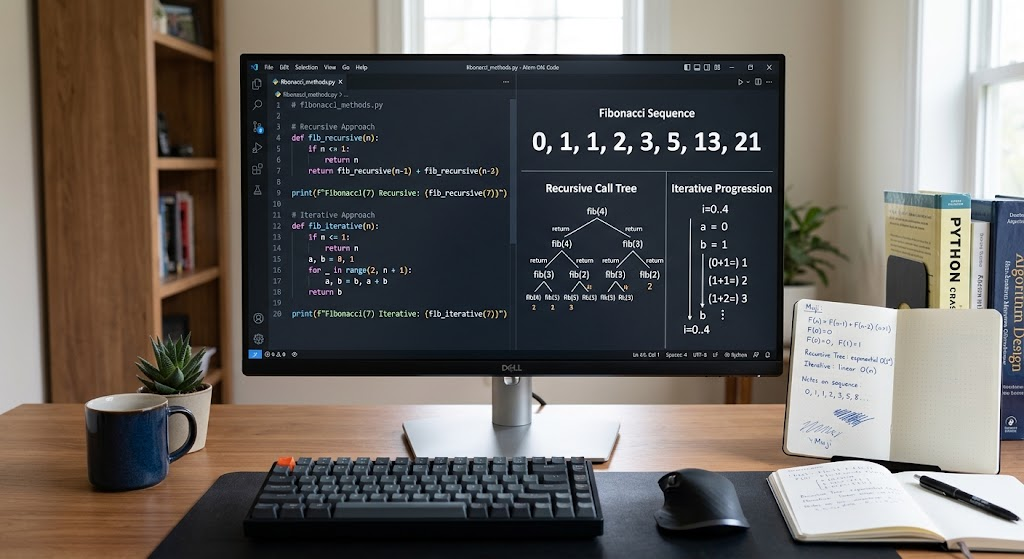
The Fibonacci sequence is a series of numbers in which each number after the first two numbers is the sum of the last two numbers. The sequence starts with 0 and 1, and the common version is 0, 1, 1, 2, 3, 5, 8, etc. Of course, the mathematical definition lends itself to recursion, as each Fibonacci number is defined in terms of two directly preceding Fibonacci numbers. But a simple recursive solution does lots of recomputation. For instance, the calculation of the nth Fibonacci may be made on several branches of function calls, all of which arrive at the same number that was previously computed. In the simple recursive solution, the number of operations will increase exponentially. An iterative solution would save this redundant effort by keeping the last two terms and renaming them as it goes through the sequence. Both methods will give the same result, although the iterative method may be more efficient if no other recursive data structure is needed to compute a single fibonacci number.
def fibonacci_recursive(n):
if n < 0:
Raises ValueError if n is negative.
if n < 2:
return n
return fibonacci_recursive(n – 1) + fibonacci_recursive(n – 2)
def fibonacci_iterative(n):
if n < 0:
Raise ValueError(‘n must be non-negative’)
previous, current = 0, 1
for _ in range(n):
previous = current, current = previous + current
return previous
print(fibonacci_recursive(6)) # Output: 8
print(fibonacci_iterative(6)) # Output: 8
The recursive version is a direct implementation of the mathematical definition, and is inefficient for large n because it calculates the same values over and over again. It has exponential time complexity (O(2ⁿ) upper bound) and a maximum call stack depth of O(n). The iterative implementation computes the same sequence using two variables and has time complexity O(n) with a constant space of O(1) if only one Fibonacci value is needed. This example illustrates the importance of more than just understanding the structure of an algorithm. The programmer should also take into account the amount of work the implementation is intended to undertake. When repeated calculations would otherwise take a long time to process, an optimized recursive method with memoization or iteration may be better alternatives to a natural starting point of recursion.
Tree Traversal
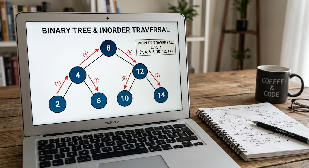
Tree is a hierarchical data structure made up of nodes related by parent-child relationships. Trees are used to model file systems, organizational hierarchies, decision making processes, and many other hierarchical representations of data. Traversing a tree involves visiting the nodes of the tree in a specific order like preorder, inorder or postorder traversal of the binary tree. A key application of recursion is in traversing a tree, where the tree itself can be viewed as a smaller tree that is recursively traversed according to the same rules as the original. A recursive traversal function can be used to visit a node then recurse into the nodes for which it is the relevant child node. The algorithm is not too complex and easy to read, as it does closely mimic the recursive definition of a tree. Very deep trees, however, can result in a considerable number of nested function calls. An iterative traversal can then prevent this issue, by maintaining a stack or queue of nodes that have yet to be traversed.
class Node:
def __init__(self, value, left=None, right=None):
self.value = value
self.left = left
self.right = right
def inorder_recursive(node):
if node is None:
return
inorder_recursive(node.left)
print(node.value)
inorder_recursive(node.right)
root = Node(
2,
left=Node(1),
right=Node(3)
)
inorder_recursive(root)
In this example, inorder traversal visits the left subtree, prints out the value of the node and then visits the right subtree. If the tree has the values of one, two, three, the output will be 1, 2, 3. This is used to prevent the function from trying to process a node that doesn’t exist, as the base case. This implementation is easy to do, using recursion: the same function can do the same work on the root as it does on each subtree. In a normal iterative version, a stack would be explicitly used to keep track of nodes as traversing the tree. Recursive traversal may be suitable for balanced trees; however, if the tree is very deep, the complexity of the recursive traversal algorithm may cause it to fail due to a runtime recursion limit. An iterative implementation might be more appropriate if the maximum depth of the trees is not known, or if the program has to process large, deeply nested data structures.
Searching Algorithms
Searching Algorithms look for a specific element in a set of elements. Linear search is checking the elements in the collection one by one until the target element is located or the collection is exhausted. Can be done with a loop or recursive function, but typically it is easier to do with a loop. Another popular technique is binary search which is applied to collections that are already sorted, and which involves repeatedly testing the element in the middle of the collection and removing half of the collection from consideration. Recursive binary search: It will call itself on the appropriate half of the collection; iterative binary version: It will change the lower and upper limits inside a loop. When properly implemented, both versions can be done in O(log n) time since the search space is cut in half each step. The iterative version usually requires O(1) amount of auxiliary space, whereas a simple recursive version requires O(log n) amount of stack space. If memory is limited, iterative binary search is a good alternative to recursive binary search.
def binary_search_iterative(numbers, target):
left = 0
right = len(numbers) – 1
while left <= right:
middle = (left + right) // 2
if numbers[middle] == target:
return middle
if numbers[middle] < target:
left = middle + 1
else:
right = middle – 1
return -1
numbers = [2, 4, 6, 8, 10, 12]
print(binary_search_iterative(numbers, 8)) # Output: 3
print(binary_search_iterative(numbers, 7)) # Output: -1
The binary search implementation starts with a search index starting at first and ending at last. In each step, it checks the middle element and compares the value at the mid index with the desired value. If it is equal to, the function returns the index. When the middle number is less than the target number, the lower bound will slide to the right of the middle; when it is greater than the target number, the upper bound will slide to the left of the middle. Loop terminates when the target is detected or search limits are exceeded. If the target is not found in the collection, then -1 is returned. This example is one of the uses of iteration for algorithms that have few variables that are repeatedly modified. The iterative is correct too, but recursive calls would use extra space on the call stack.
Common Risks and Challenges
Recursion and iteration can lead to errors in their stopping conditions and/or their logic. A recursive algorithm must have a base case and a recursive case that takes the problem closer to the base case. If either of these is not implemented or is missing, the function can call itself indefinitely until it hits the recursion limit of the runtime or the maximum stack depth. The other type of risk in iterative algorithms is that the loop condition may be wrong or a variable may never change correctly, leading to an infinite loop.
This loop can take time to process and cause a program to fail to perform its intended action. For both approaches, programmers are expected to try both simple and extreme values, wherever applicable, as well as invalid values. In recursive procedures, they should check that all possible recursive calls lead to a base case. They should test the loop to see whether it runs as intended and whether the condition for loop termination is correct.
Understanding Stack Overflow
Stack overflow will happen if the program calls too many functions. This is a typical problem in recursive algorithms, such as when the function is called too many times or if it does not terminate correctly. The recursive procedure that keeps calling itself with the same argument will never terminate, for instance. If the recursive logic is correct, but the recursive calls are very deep, it can cause the environment to exceed the recursion depth that it supports.
The error can cause the program to be halted before it reaches the desired calculation. To minimize this risk, the developer can verify the base cases, make sure that every recursive call advances, and look at an iterative option for the task if it might be very recursive. Certain recursive stack frames can be eliminated because of tail call optimization in some programming languages, but this is not available in all languages. It is best for programmers to know how their language handles recursive calls to know that they are not always optimized.
Avoiding Infinite Loops
Infinite loops are loops that run forever without reaching the termination condition of the program. This can occur when no counter is incremented, if a condition is incorrectly written, or if the loop is going through the same state over and over again with no improvement. For instance, a counter in a while loop that is never incremented by one which is less than ten would loop forever if the initial value of the counter is less than ten. These mistakes can lead to slow or unresponsive applications, or applications using more computing power than is necessary.
Programmers should recognize what changes in each iteration and make sure that the change gets them closer to termination to prevent these issues. It is also necessary to test the boundary conditions – that is, empty collection or missing target value – since a loop might execute properly for normal data but fail to run under these conditions. To make sure iterative algorithms do their jobs correctly, loop conditions are clarified, variable changes are carefully selected, and test cases are strategically selected.
When to Use Recursion
Recursion is a more appropriate solution if a problem is naturally decomposed into smaller problems of the same type. Some examples are traversing trees, exploring hierarchical structures, processing nested expressions, and implementing some divide and conquer algorithms. It can simplify things when the operations are complicated since it breaks down the overall task into smaller operations. Recursion is also useful if the mathematical problem has a naturally recursive definition which does not result in an unacceptable performance or memory cost when implemented recursively.
Developers need to consider the maximum depth of recursion that could occur and decide if multiple function calls are necessary in the environment they are developing for. Recursive solutions to problems that solve the same subproblems over and over can be made more efficient by using techniques like memoization. Recursion can be used to generate clear and maintainable code, which would otherwise require more complex control structures, when the recursion is similar in structure to the problem, and the depth is not too great.
When to Use Iteration
Iteration is typically a good idea when an algorithm involves simple repetition, counting, processing a sequence, or updating a few variables. Loops can be used to express tasks like calculating a running total, searching a list, processing records and generating a sequence, among others, quite clearly. Iterative algorithms are also usually suitable for situations where memory is an issue as they may not require the size of the stack to grow when running the recursive procedures several times. They are very helpful if the input can be large or if the depth of a problem can be hard to determine.
Iteration isn’t always the easiest solution to all problems, though. For a recursive implementation, if a complicated tree traversal or a deeply-nested data-processing operation is performed, explicit stacks and bookkeeping might be necessary. Before making a decision, the programmer should analyze the clarity and resource usage of each of them. When the pattern for repeating a set of instructions is simple to describe, iteration is often an efficient and predictable solution to many of the everyday programming problems.
Conclusion
Recursion and iteration are two basic methods of designing algorithms that perform repeated operations, but differ in the manner in which they organize the repeat. Recursion: A recursive function is a function that solves a problem by calling itself with a smaller instance of the problem, with base cases to halt further recursion. Iteration is used to repeat instructions within loops that are terminated when certain conditions are met. Both methods can be used to solve problems like factorial, fibonacci sequence, traversing a tree and searching, but their performance and memory usage may differ greatly.
Recursive algorithms are good for hierarchical structures and problems that naturally break down into smaller versions of themselves, iterative algorithms are better for simple repetition and problems where call stack usage is a concern. Recognizing these differences can help programmers make informed choices when designing and building their systems with clarity, efficiency, and reliability. Recursion and iteration are not mutually exclusive methods with a single best solution, but should be used in the situations where they will be most useful.


