Introduction
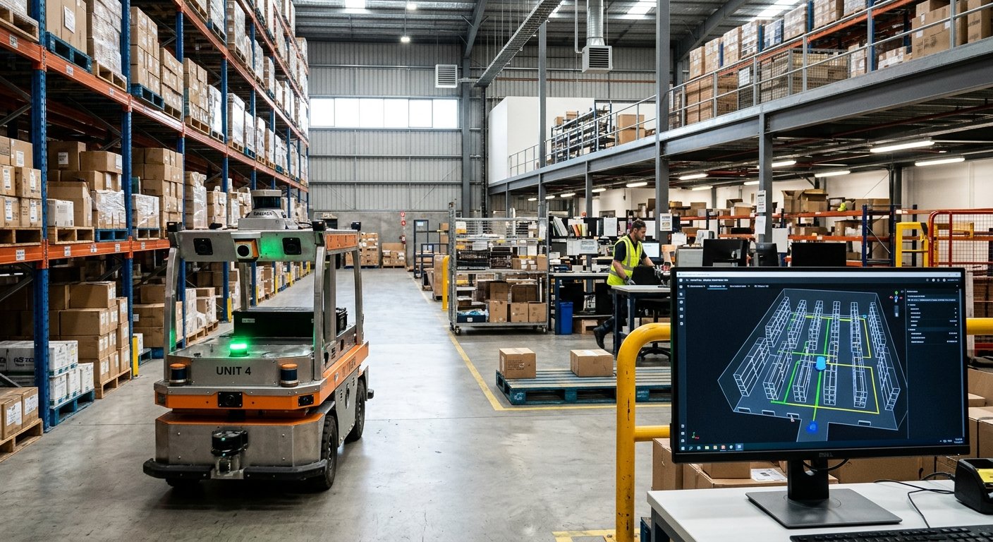
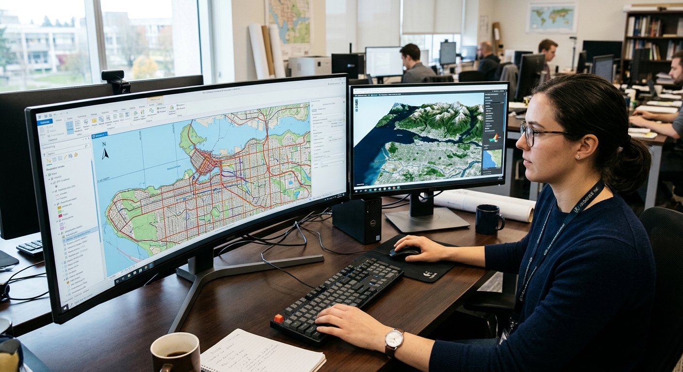
Computational geometry is a key part of computer science and consists of creating efficient algorithms to solve problems based around geometry. The algorithms take mathematical concepts and translate them into code for the computer to process. This can be used to find distances, intersections and help understand spatial relationships. This can be explored further through Computational Geometry Algorithms. Computational geometry is used within computer graphics, robotics, GIS, CAD, image processing and AI. For example, navigation apps can use this to find the shortest route between two points. Computer Graphics can use this to build realistic 3D scenes. It gives students the mathematical knowledge needed to solve complex spatial problems efficiently.
Computational geometry is an important concept to understand. A lot of real life problems require finding out where objects are located, if they overlap, how far apart objects are and how to divide a set of objects into smaller sets. When working with thousands or millions of geometric data, this can become very inefficient using simple comparisons. Therefore, computational geometry can be used to provide a structured approach to solving these issues. Understanding techniques such as Convex hulls, Voronoi diagrams, Delaunay Triangulation, Line Segment Intersections, Point Location, Polygon Triangulation and Closest Pair can give students a greater understanding of how to apply mathematical concepts.
1. Understanding the Basics of Computational Geometry
Computational geometry is concerned with analysing algorithms that solve problems related to geometry. The most common geometrical objects are points, line segments, polygons and circles. Points are exact locations, line segments are created by connecting two points together. Polygons are shapes made up of line segments connected together to make a closed shape. Circles are made up of points that are a fixed distance from the center point. These objects are typically shown with coordinates. A point in a 2d plane can be shown as (x,y). This can be inputted into a computer program which can work out distances, orientation, intersections.
Understanding how the algorithms work using the geometric information is an important concept to learn. For example, having three points shown with coordinates, a computer can work out if they are all in line by using mathematical calculations. Or if a point is inside a polygon by looking at the points orientation. Although simple, this can be the basis for more complex algorithms. It is also important to understand computational complexity. This is how much resources an algorithm will use when given more input data. Common complexities are O(n), O(n log n) and O(n²). Knowing these concepts will help compare the different algorithms for solving geometry problems.
2. Convex Hull Algorithms
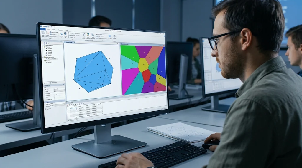
A convex hull is the smallest convex polygon that can contain all the points. A convex shape is one where a straight line drawn between any two points will stay inside the shape. An easy way to understand what a convex hull is, is if you place multiple nails onto a wooden board and stretch a rubber band around all of them. When you let go of the rubber band, it will form a boundary around the outermost nails. This is the convex hull. Any points inside the convex hull will not contribute to the outer shape. Convex hulls are important as they help computers find the outer boundaries of spatial data. This can be used in image processing, collision detection, geographical analysis, pattern recognition and computer graphics.
There are various algorithms to calculate the convex hull of a set of points. One popular algorithm is the Graham scan. This algorithm sorts the points based on their polar angle to a chosen starting point. Once the points are sorted they are processed using a stack to ensure that points that would cause an inward turn are removed. This will continue until all points have been checked and the convex hull has been formed. This has a time complexity of O(n log n) due to the initial sorting step. The scanning step has a complexity of O(n). Another algorithm is the Jarvis march also known as the gift wrapping algorithm. This works by selecting the next point on the convex hull based on the orientation of the points. It has a time complexity of O(nh) where n is the total number of points and h is the points on the convex hull. This can be useful if there aren’t many points on the convex hull.
Real-Life Applications of Convex Hull Algorithms
Convex hull algorithms can be applied to many real life situations. In computer graphics it helps find the outer boundaries of objects. It can also be used for detecting collisions between moving objects. In robotics, convex hulls can be used to show the approximate boundaries of obstacles. This helps robots understand how their environment is laid out. In GIS, convex hulls can be used to find the smallest convex area that can contain a set of locations.
For example, imagine a city authority collects the coordinates of ten public facilities. They want to know the general area that all these locations are in. A convex hull algorithm can be used to calculate the outer boundary. This shows how a simple concept can become a useful tool.
3. Voronoi Diagrams
A Voronoi diagram is a geometric structure that splits a plane into regions. Each region contains all points that are closer to a specific site than any other site. The boundary between adjacent regions will be where points are equidistant to two or more sites. For example, if there are multiple hospitals in a town, a Voronoi diagram can be used to split the town into regions. This will show which hospital is the closest to each location. If someone was in a specific region, then they will be closer to the corresponding hospital than any other hospital in the diagram.
To create a Voronoi diagram, you need to calculate the regions for a set of sites. A common method is using a perpendicular bisector between two sites. This is a line that divides the space between two points. Any points along this line will be equidistant to both points. Combining these boundaries and identifying which sections apply to adjacent sites can be used to create a full Voronoi diagram. For a set of n points in a plane, a Voronoi diagram will have O(n) edges and vertices. This can be created efficiently using Fortune’s Algorithm. This has a time complexity of O(n log n) and a space complexity of O(n). This algorithm works by sweeping a line across the plane and keeping track of some geometric events.
Real-Life Applications of Voronoi Diagrams
Voronoi diagrams can be used for many real life applications. In geographical analysis, it can help determine which mobile tower is the closest to certain locations. This can be used when initially designing a network. In agriculture, it can help split farmland into regions based on monitoring stations. This allows farmers to analyse soil conditions.
Emergency services can use Voronoi diagrams to estimate which fire station, hospital or emergency facility is closest. For example, if a government agency wanted to build new healthcare facilities they could look at how the hospitals are distributed. They can see which areas are relatively far away from any services. Although in real life factors like roads, traffic and capacity of the facilities should be considered, Voronoi diagrams can be used as a starting point.
4. Delaunay Triangulation
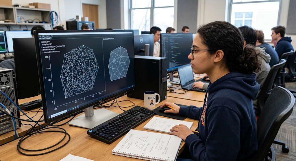
A Delaunay Triangulation is a method of breaking a set of points into triangles. A valid Delaunay Triangulation will have no other input points inside the circumcircle of the triangle. A circumcircle is a circle that passes through all three vertices of the triangle. This means triangles can be created that have good properties. This also means the triangles won’t be too skinny. Delaunay Triangulation is closely related to Voronoi diagrams as they are a dual of each other. This means that the sites of the Voronoi diagram are the vertices of the Delaunay Triangulation. Adjacent regions of the Voronoi diagram will be connected by edges. This means that both can be useful for analysing spatial data.
There are multiple algorithms that can be used to create a Delaunay Triangulation. These include incremental insertion, divide and conquer and edge flipping. Incremental insertion creates a basic triangulation and then inserts points one-by-one. As each point is added, the adjacent triangles are adjusted if the Delaunay condition is broken. Edge flipping is used to improve the triangulation by changing the edges to a better configuration. Divide and conquer works by splitting the points into smaller groups. Each group is triangulated and then combined. Under normal assumptions, efficient algorithms can be used to create a Delaunay Triangulation with a time complexity of O(n log n). This will have O(n) edges.
Real-Life Applications of Delaunay Triangulation
Delaunay Triangulation is used to create triangular meshes in computer graphics, geographical modelling, scientific simulations and 3D surface reconstruction. In computer graphics, it can help create triangular meshes. In geography it can be used to create a terrain model. For example, environmental researchers may collect elevation data from various locations.
They can use Delaunay Triangulation to connect these points. This can help with calculations relating to the shape of the terrain, gradients and changes in elevation. Engineers can use triangulated meshes in finite element analysis. This involves splitting complex physical structures into smaller elements. The ability to form useful triangular meshes makes Delaunay Triangulation an important concept.
5. Line Segment Intersection Algorithms
Line Segment Intersection algorithms are used to find if two or more line segments intersect. This is an important concept to understand as geometric objects often interact in computer applications. For example, in computer graphics you might want to know if two lines in a drawing intersect. Or in a map application, you may want to know which road segments intersect. To check if two lines intersect, you can look at the orientation of the end points of each line segment. Orientation tells us if three points make a clockwise turn, anti-clockwise turn or if the points are colinear. By looking at the orientation of the relevant points we can determine if the line segments intersect. Special cases such as collinear segments and shared end points must also be considered.
Checking every possible pair for n line segments will have a time complexity of O(n²). This is because there will be roughly n(n-1)/2 pairs to check. This isn’t too bad for small data sets but can be inefficient for large data sets with thousands of line segments. A more efficient algorithm can be used to find intersections of multiple line segments. The Bentley-Ottmann algorithm uses a sweep line approach. This works by sweeping a line across the plane. As the line sweeps across, it keeps track of the segments in a sorted order. This focuses on adjacent segments and looks at key events. This will have a typical time complexity of O((n+k) log n) where n is the number of segments and k is the number of intersections found. This assumes that the general position assumptions are met and the algorithm is implemented properly.
Real-Life Applications of Line Segment Intersection
Line segment intersection algorithms can be very useful in computer graphics, CAD, GIS and digital mapping. In a graphics application, it can help to find intersections of lines in a drawing. In CAD, intersection calculations can be used to find how different edges and parts relate to each other when designing mechanical parts, buildings and more.
In digital mapping, it can help look at road networks, connections and geographical boundaries. For example, in a mapping application you may want to know where roads intersect so you can create a connected transport network. Efficient intersection detection can help the software handle complex maps.
6. Point Location Algorithms
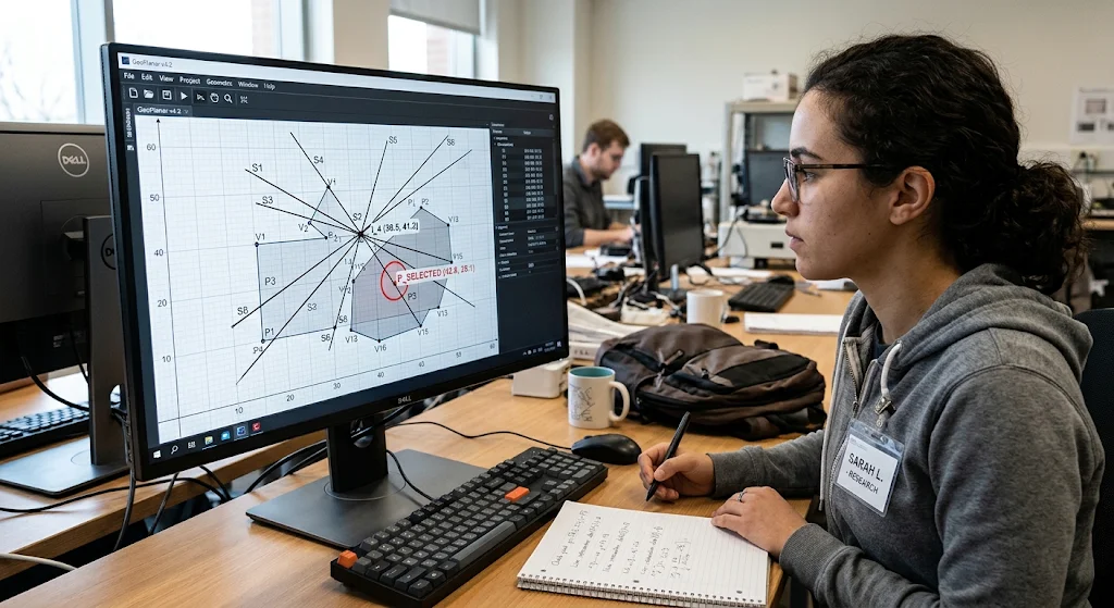
Point location is the problem of finding which region of a subdivision a query point lies in. A subdivision is when a geometric space is split into smaller regions using boundaries. For example, in a digital map a country may be split into states, cities or administrative areas. If a user clicks on a location on the map, a point location algorithm can tell you which region the point is in. This is an important concept to understand as many applications will want to find out which area of the geography/geometry a specific coordinate relates to. A simple method to do this would be to check each region until the correct one is found. This can become inefficient when there are lots of regions in the subdivision.
More efficient algorithms exist that arrange the data in a certain way to enable faster searching. Trapezoidal maps can be used to split the planar subdivision into simpler regions to make searching easier. Hierarchical searching can also be used to help eliminate large amounts of the subdivision. If a planar subdivision has n edges, a good point location structure can often be created in O(n log n) and queries can be answered in O(log n). Some more advanced methods can give faster expected query times but will require extra pre-processing. This demonstrates an important concept in algorithms. Spending time organising your data can greatly reduce the cost of doing repeated operations.
Real-Life Applications of Point Location
Point location algorithms are commonly used in digital mapping, GIS, computer graphics and spatial databases. In GIS applications they can help determine which area a coordinate is in. In computer graphics, point location can be used to determine which part of the scene the selected point is in. Spatial databases also use similar techniques to find records that relate to certain geographical areas. For example, in a delivery application the city may be split into multiple delivery zones.
When a customer inputs an address, this can be converted into a set of geographical coordinates. A point location algorithm can be used to find out which delivery zone it belongs to. This means the application can quickly find the relevant service information without having to search through every zone. Point location is therefore an important technique for applications that have lots of queries relating to geography.
7. Polygon Triangulation Algorithms
Polygon Triangulation involves dividing a polygon into triangles. This will result in non-overlapping triangles that completely fill the polygon. This is an important concept as triangles are a simple shape that can be processed efficiently by the computer. Complex polygons with lots of vertices can be difficult to analyse, but dividing them into triangles can make things easier. Computer graphics applications use triangulation to turn polygonal surfaces into something that can be rendered by the graphics hardware. Engineering applications use triangulation to perform calculations on complex surfaces. A simple example would be a rectangular polygon. This can easily be split into two triangles by drawing a line between opposite vertices. More complex polygons will require algorithms to find valid diagonals that don’t cause the triangles to go outside of the shape.
There are multiple algorithms that can be used to triangulate a polygon. For simple polygons with n vertices, the ear clipping algorithm can be used. This will repeatedly find ears. An ear is made up of three consecutive vertices of the polygon with no other vertices inside the triangle. The middle vertex is then removed. This continues until there is only a triangle left. A simple implementation will have a time complexity of O(n²). However, using specialised data structures can reduce the actual cost. Monotone polygon triangulation can also be used. This involves triangulating a y-monotone polygon in O(n) time. This can be done by ordering the vertices in the right way and using a stack based approach. All simple polygons with n vertices can be triangulated into exactly n-2 triangles. This gives a predictable way to convert polygon boundaries into simpler shapes.
Real-Life Applications of Polygon Triangulation
Polygon triangulation plays an important role in computer graphics, games, geographical modelling and engineering. 3D graphics systems often use triangular meshes to represent complex surfaces. This is because they are easy to manipulate, shade and render. Games engines also use triangulation to convert polygonal objects into something that can be rendered. In GIS, polygon triangulation can help break geographical regions down into smaller pieces.
Engineering software uses triangular elements to perform calculations on complex surfaces. For example, an architectural design application may represent an irregular surface of a building using triangles. This means calculations can be performed. This shows how polygon triangulation is an essential technique to convert complex shapes into something that can be processed by the computer more efficiently.
8. Closest Pair Algorithms
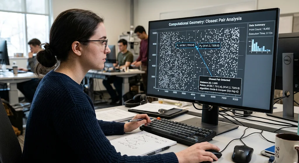
The closest pair problem is a problem which asks us to find the two closest points within a set of points. Although this seems like a simple problem it can be difficult to create efficient algorithms to find the solution. The simplest way to solve this problem is by brute force. We compare every pair and find the smallest distance. This has a time complexity of O(n² ). For n points there will be roughly n(n-1)/2 pairs of points. This can cause inefficiencies for larger sets. Imagine if you were using a system to track the locations of thousands of delivery vehicles. You would have to calculate the distance between many pairs of vehicles to find the two closest ones.
A more efficient method is to divide and conquer. We sort the points based on their x values and split them into two roughly equal halves. We then recursively find the closest pair in each half. As the closest pair could be one from each half we look at all the points around the dividing line. We sort these points based on their y value and due to careful selection we don’t look at all of the pairs. This gives us a time complexity of O(n log n). This is much more efficient than the brute force method for large data sets. It shows how breaking down a difficult problem can help to reduce the amount of computation required to get an accurate answer.
Real-Life Uses of Closest Pair Algorithms
Closest pair algorithms can be useful within robotics, GIS, Computer Vision, transportation and scientific research. Within robotics they can help find objects which are close together or help to find the shortest distance between important measurements. Within GIS they can help find facilities, locations or monitoring stations which are close together.
Within computer vision they can help with similar distance calculations when comparing feature points. An environmental monitoring organisation may want to find out which two of their observation stations are the closest. A closest pair algorithm can help do this efficiently. Although real life situations may have extra distance calculations and constraints, it shows us an important method to efficiently analyse spatial data.
9. Comparing Main Computational Geometry Algorithms
Understanding the differences between these algorithms can help students understand what algorithm to use for specific problems. There are several algorithms which deal with points, lines and polygons but each have their own purpose. The convex hull algorithm will find the outer boundary of a set of points. The Voronoi diagram will partition space based on the distance to sites. The Delaunay triangulation will join points into triangles. The line segment intersection algorithm will find where lines intersect. The point location algorithm will find which region contains a certain point. Polygon triangulation will split complex shapes into triangles. Finally the closest pair algorithm will find the two closest points. They also have different time complexities as they use different methods such as sorting, recursion, sweep line and spatial searches.
| Algorithm | Purpose | Time Complexity |
| Graham’s Scan | Convex Hull | O(n log n) |
| Jarvis March | Convex Hull | O(nh) |
| Voronoi Diagram (Fortune’s Algorithm) | Partition Space Based On Closest Sites | O(n log n) |
| Delaunay Triangulation | Join Points Into Triangles | O(n log n) |
| Bentley-Ottmann Algorithm | Report Line Segment Intersection | O((n + k) log n) |
| Point Location | Find Region Containing Point | O(log n) with proper pre-processing |
| Ear Clipping | Split Simple Polygon Into Triangles | O(n²) |
| Closest Pair Divide and Conquer | Find Two Closest Points | O(n log n) |
These are typical time complexities based on assumptions about the input data and how the algorithm was implemented. n represents the number of points/segments/polygon vertices depending on the problem. In the Bentley-Ottmann Algorithm k represents the number of intersections being reported and h represents the number of vertices in a convex hull. It is important to note that just because an algorithm has a certain computational complexity doesn’t mean it will be the best choice. Factors such as memory usage, distribution of data, precision of data, quality of implementation and frequency of queries can all affect performance. Students should consider these factors when choosing a computational geometry method.
10. Difficulties with Implementing Computational Geometry Algorithms
Although computational geometry algorithms can be useful there are several issues we may face when implementing them. One issue is precision. Many numbers are stored as floating point values within computers. This can lead to small rounding errors. When solving a problem with geometry these small errors can cause issues when determining if two points are the same, if lines intersect or if a point is inside a polygon. This can cause incorrect results. If we are working with almost parallel lines, very small distances or large numbers we will face issues. We need to use appropriate numeric types and reliable predicates to help make important decisions. Using precise arithmetic and careful tolerance methods can help reduce any issues. Depending on the application we may need to use different methods.
We also need to consider edge cases. For example the convex hull algorithm must take into consideration multiple points lying on the same line. The line intersection algorithm must take into consideration overlapping lines and lines with the same endpoints. The Voronoi diagram and Delaunay triangulation may also need consideration if there are multiple points with the same distance or four or more points lying on the same circle. When working with very large data sets we may also need to worry about memory usage and processing time. Some applications may also require frequent updates so new points/geometric objects are constantly being added and removed. To create efficient solutions we need to understand how to create reliable data structures. Computer science students need to understand how to test edge cases and find a balance between precision and performance.
Conclusion
Computational geometry provides vital techniques to solve problems with points, lines, polygons and spatial data. We can use algorithms such as convex hulls, Voronoi diagrams, Delaunay triangulation, line segment intersection, point location, polygon triangulation and closest pair detection to show how mathematical principles can be used to create efficient solutions. Although each technique solves a different problem they all have the aim of accurately processing spatial data with minimal unnecessary calculations. These techniques can be used within computer graphics, robotics, mapping, GIS, engineering, research and AI. Understanding these techniques can help students understand how computers process and represent spatial data.
Learning about computational geometry can be beneficial for computer science students. It can help improve problem solving skills, mathematical reasoning and understanding of algorithm efficiency. By understanding how different algorithms work, comparing their time complexity and playing around with examples using simple coordinate values we can better understand more abstract geometric concepts. If you would like to learn more about this topic you can refer to this academic resource titled Computational Geometry Algorithms. As technology continues to develop, computational geometry will continue to play an important role in creating intelligent systems which can interpret, organise and interact with spatial data.