Introduction
One of the most important skills to learn in programming is how to solve complex problems efficiently. With more data being processed, basic solutions can be inefficient, take up more resources and become harder to manage. This is where the divide and conquer algorithm comes in. Divide and conquer is an algorithm design technique that splits a problem into smaller subproblems, solves each subproblem separately, and then combines the results together to solve the whole problem.
Some of the most important algorithms use divide and conquer such as merge sort, quicksort and binary search. By reducing the amount of work that needs to be done at each step, divide and conquer can make your code more efficient. Overall understanding how divide and conquer works can help you as a programmer to come up with more efficient strategies to solve a problem, choose the right algorithm to use and write code that works well with large amounts of data.
What Is the Divide and Conquer Technique?
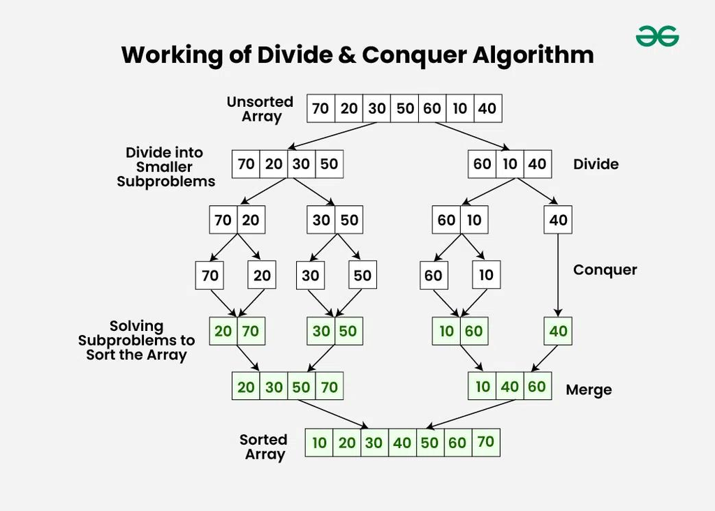
The divide and conquer algorithm is an algorithm design paradigm that divides a problem up into smaller instances of the same problem. This makes the problem easier to understand and solve as the algorithm will split the problem into smaller chunks. Usually, these smaller problems are independent of each other. The results from each problem are combined to give the solution to the original problem. Divide and conquer works best when there is some structure to the problem that can be continuously divided.
It is also closely related to recursion however not all divide and conquer algorithms will use recursion. Recursion is when a function calls itself to solve a smaller instance of the original problem. This will continue to split the problem until a base case is reached. The base case is when the problem can be solved easily. From this point the function will start to return values and combine them. This makes the problem solving process very structured.
Three Main Steps of Divide and Conquer
There are 3 main steps to the divide and conquer algorithm. They divide, conquer and combine. Depending on the algorithm, these steps will be implemented differently. Knowing these steps can help make it easier for developers to see if a problem can benefit from divide and conquer.
- Divide
The first step is to split the original problem into smaller subproblems. These subproblems should be similar to the original problem but smaller. For example, if you are trying to sort a list of hundreds of numbers you can split this list into two smaller sections.
You can then continue to split each section until there is only one item in each section. How you split the problem will depend on the algorithm you are using. Some algorithms will split the data evenly whereas others will split unevenly based on certain conditions. The aim is to make the problem smaller and manageable.
- Conquer
Once the problem has been split into smaller subproblems we want to solve each of these. If the divide and conquer algorithm uses recursion, this process will repeat on each smaller section until the base case is reached.
The base case is when the problem can be easily solved. For example, if you only have one item in your list then it is already sorted. Once all the smaller problems have reached their base case they can be solved.
- Combine
Once the smaller problems have been solved we can now combine their solutions to give us the solution to the original problem. How this works depends on the algorithm. In merge sort we will combine the sorted sections together to create larger sorted sections.
Other algorithms may pick the best result or add everything together. Some divide and conquer algorithms will have a lot of work to do in this stage whereas others won’t have much to do. How efficient this stage is can affect the overall efficiency of your algorithm.
Recursion
A key concept in programming is recursion. Many divide and conquer algorithms use recursion. This allows a function to call itself using a smaller input. This means we don’t have to write instructions for every possible problem size. We can write one function that will handle the general process. This function will continue to apply itself to smaller inputs, giving a more organised solution. This is useful when the problem contains smaller versions of itself. For example sorting a list, searching through a collection or working with hierarchical data.
Every recursive function will have a base case and recursive case. The base case tells the function when to stop calling itself. The recursive case is when the problem gets smaller with each call. If you don’t have a suitable base case the recursion will go on forever until the program encounters an error such as a stack overflow. Each time the function calls itself it creates a new stack frame. Once the base case is reached the function will start returning the results from each call. When creating divide and conquer algorithms you must consider how the recursion works and how much memory it will use.
Example of a Recursive Function
One simple example is calculating the factorial of a positive integer. The factorial of a number is the product of all positive integers from that number down to one. This can be solved using recursion as to calculate the factorial of a number you must calculate the factorial of a smaller number.
def factorial(n): if n == 0 or n == 1: return 1 return n * factorial(n-1)print(factorial(5))
The function will keep calling itself with a smaller value until it reaches 0 or 1. The base case will return 1. The previous calls will then multiply their values together to give a result of 120. This isn’t a typical divide and conquer algorithm as there is only one smaller recursive subproblem however it shows how recursion works. Understanding this concept will give you a good foundation for learning about algorithms that split the problem into multiple smaller sections.
Merge Sort
One of the most obvious examples of a divide and conquer algorithm is merge sort. This is a sorting algorithm that will sort the elements in either ascending or descending order. It does this by continually splitting the list into smaller sections.
These sections are then sorted and merged. This makes it very useful for large datasets as the time complexity will always be predictable. It is also stable meaning if there are duplicate values they will maintain their original order.
How Merge Sort Works
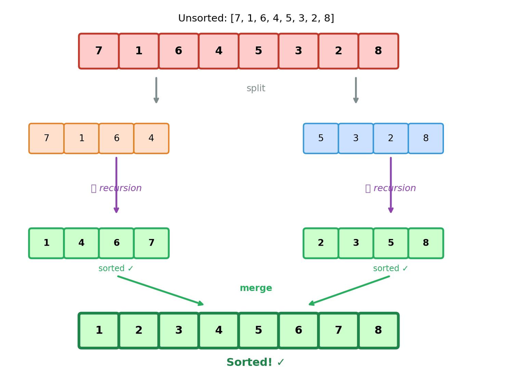
Merge sort works in a very simple way. Firstly the original list will be split into 2 smaller halves. Each half will be split into smaller sections until each section only contains one item. Since this is already sorted these will be the base case of the algorithm. The algorithm will now start to merge the sections together. The items will be compared and put into the correct order. As the sections get merged together they will become larger sorted sections. This means merge sort can be used for large collections.
Let’s look at an example. Our list of numbers is:
[38, 12, 27, 43, 9, 31, 18, 25]
The algorithm will split the list into 2 halves.
- Left section: [38, 12, 27, 43]
- Right section: [9, 31, 18, 25]
These will be further split until each section only contains one number. The numbers will then be compared and merged to create sorted pairs. These pairs will then be merged to create larger sorted sections. The final list will be:
[9, 12, 18, 25, 27, 31, 38, 43]
Time and Space Complexity
Merge sort has a time complexity of O(n log n) in the best, average and worst case. The log part of the equation refers to how many times the input can be divided by 2. The n part refers to how much work is done when merging. Since the list is split into roughly even sections there will be around log 2 (n) divisions. At each division all n items will be merged. This gives us a time complexity of O(n log n). This is very useful as it will always be predictable. This makes it useful for large collections.
Merge sort also requires extra memory if it is implemented using arrays. It will have an auxiliary space complexity of O(n). This can make it less suitable for very memory restricted situations. Despite this it can still be very useful as it provides a reliable performance. It is a commonly talked about algorithm in computer science as it shows how recursion can be used with problem solving and complexity analysis.
Quicksort
Another popular sorting algorithm that uses divide and conquer is quicksort. Like merge sort it will split the collection into smaller sections. However it will use a selected item known as a pivot to split the collection. Items will then be moved around depending on if they are smaller or larger than the pivot.
Once this has happened the sections will be sorted recursively. Unlike merge sort there is no merging stage as the pivot will be in the correct position once the collection is split. This makes quicksort very efficient in many situations.
How Quicksort Works
The first thing quicksort will do is select a pivot. This can be the first, last, middle item or selected using a strategy such as randomly. The rest of the items will then be split based on their values. Items smaller than the pivot will be on one side and items larger than the pivot will be on the other. The pivot will now be in its correct position. The process will then be repeated recursively on the sections on either side of the pivot until there is only one item in each section.
Let’s look at an example. Our collection of items is:
[35, 20, 45, 10, 30, 50, 15]
We will select 30 as our pivot. This can be split into:
- Smaller items: [20, 10, 15]
- Pivot: 30
- Larger items: [35, 45, 50]
The smaller and larger sections will then be sorted. Once they have been sorted they will be arranged around our pivot to give us:
[10, 15, 20, 30, 35, 45, 50]
Time and Space Complexity
Quicksort has an average time complexity of O(n log n). This makes it very efficient for many sorting situations. How efficient this is depends on how well the pivot splits the collection. If the pivot splits the collection into fairly even sections then the problem will be reduced efficiently. However if the pivot keeps splitting the list into very uneven sections such as one section having almost all the items and the other having very few then the time complexity will be O(n 2) in the worst case. This can happen if a poor pivot selection strategy is used.
Quicksort can also be done in-place. This means it can sort the items in the original collection without needing an additional array of the same size. The average space complexity will be O(log n) due to the recursive calls. However, in the worst case the recursion can go up to O(n). Quicksort is often favoured if you want an efficient average case. However you must consider the pivot selection, recursion and the nature of the input.
Binary Search
Binary search is a searching algorithm that uses divide and conquer. It will search for a specific value in a sorted collection. Instead of searching for each item it will look at the middle item and decide which half it could be in. If the middle item is the value it is looking for then the search will end.
If it is smaller then it will continue to search the left half. If it is larger then it will continue to search the right half. This means roughly half the items will be ignored each time a comparison is made. This can make finding the value much faster than a basic linear search if the collection is large and sorted.
How Binary Search Works
The first thing the algorithm will do is find the first and last position in the sorted collection. It will then find the middle position. It will compare the value with the target. If they match then it will return the position of the target. If it is smaller then it will search the items before the middle position. If it is larger then it will search the items after the middle position. This process will continue until the target has been found or there are no more items to search. Each comparison will ignore roughly half of the remaining items. This is why binary search is so efficient.
Let’s look at an example. Our sorted collection is:
[5, 10, 15, 20, 25, 30, 35, 40, 45]
Our goal is to find the number 35. The algorithm will look at the middle item which is 25. Since it is smaller than our target we can ignore the left section. It will then look at the middle item of this section and find our target. As we only had to make a few comparisons instead of going through each item at the start this makes binary search very effective with large sorted collections.
Time and Space Complexity
Binary search has a best case time complexity of O(1) as it can find the target in the first comparison if it is in the middle. It has an average and worst case time complexity of O(log n). This is because roughly half of the search space will be ignored after each comparison. For example if there are 1024 items in the collection it will only take around 11 comparisons in the worst case. Whereas a linear search may take 1024 comparisons. This becomes more important the larger the collection gets.
Depending on how the algorithm is implemented it will have a different space complexity. If it is implemented iteratively then it will have a space complexity of O(1) as there will only be a few variables. However, if it is implemented recursively then it will have a space complexity of O(log n) in the worst case. A downfall of binary search is that it requires the data to be sorted. If the collection isn’t sorted you may have to sort it before searching. You should consider whether it would be worth sorting the data.
Time Complexity
Time complexity refers to how long an algorithm will take to run based on the size of the input. This is often represented using Big O Notation. Divide and conquer algorithms are often analysed by seeing how many smaller subproblems are created, how large they are and how much work is needed to split and combine them. This can help you as a developer understand whether the algorithm will remain efficient when there is more data to process. It can also give you a basis to compare different ways of solving the problem.
A common way to represent the runtime of a divide and conquer algorithm is using a recurrence relation. This is when the time taken to solve the problem is represented in terms of the time taken to solve the smaller subproblems. A general recurrence relation can be written as:
T(n)=aT(n/b)+f(n)
Where n is the size of the input, a is the number of subproblems, n/b is the approximate size of each subproblem and f(n) is the extra work done. This can be useful as it allows you to analyse recursive algorithms. There is a method called the Master Theorem which can be used to solve many recurrences and determine their asymptotic time complexity.
Common Complexity Types
Understanding how to calculate common complexity types can help a developer determine how efficient a divide and conquer algorithm will perform.
| Complexity | Meaning | Example |
| O(1) | Constant | Accessing an index in an array |
| O(log n) | Logarithmic | Binary Search |
| O(n) | Linear | Iterating through an array |
| O(n log n) | Linearithmic | Merge Sort |
| O(n²) | Quadratic | Bubble Sort |
Algorithms with a complexity of O(log n) generally run more efficiently than O(n) algorithms when there are large amounts of input. O(n log n) sorting algorithms also tend to be more efficient than O(n²) sorting algorithms when working with large datasets. However, Big O does not account for every factor that can affect an algorithm. Other factors such as the hardware, language, memory access, quality of implementation and type of input can affect how long the algorithm takes to run. A developer should consider the complexity, but also test out different algorithms.
Benefits of Divide and Conquer Algorithms
There are many benefits to using divide and conquer algorithms. The main benefit is that it can simplify complex problems by breaking them down into smaller chunks. This allows algorithms to be more easily understood, implemented and analysed. If the problem being solved is naturally recursive then it can really help. The algorithm can also be more efficient when executing as it helps reduce the amount of operations that need to occur. Algorithms like merge sort and binary search have shown that when continually reducing the size of the problem you can have very efficient algorithms.
An important benefit to this is that if the sub-problems are independent then they can be solved at the same time. This means we can utilize parallelism by having multiple processors or cores working on different aspects of the problem. For example, we can split up different parts of a large dataset and solve them. Divide and conquer can also encourage a modular approach to programming as each small operation can be created and tested individually. This makes it easier to spot errors in the algorithm, improve parts of it and keep complex software systems well maintained. However, this depends on the problem.

Drawbacks and Limitations of Divide and Conquer
Despite the benefits of divide and conquer it is not always the best way to solve a problem. There can be issues with recursion. Every time a function is called recursively it will take extra time and memory. If the problem is small or can be solved easily with iteration then using a divide and conquer algorithm could make the algorithm overly complex or inefficient. For example, if we had a small set of elements to process then using a simple loop may be more practical. So a developer should consider whether splitting the problem will help.
Some algorithms require a lot of extra memory to combine their results. Merge sort is commonly known for requiring extra memory to store the data during the merge process. Not every problem can be broken down into smaller independent sub-problems. Some problems can be dependent on each other making it difficult to split into smaller parts. Also, the combined step may take a lot of effort to do, meaning that it may not be as efficient as expected. If the problem isn’t split well then this can cause issues, for example with quicksort. Knowing what the limitations of this technique are can help a developer decide not to use it if there is a better algorithm design technique.
When to Use Divide and Conquer
The best time to use divide and conquer is when we can split the problem into smaller sub-problems that are similar to the original. The sub-problems should be easy to manage and the results from solving the sub-problem should be able to be combined to give us our final answer. Problems such as sorting, searching, mathematical calculations and processing large sets of data are common problems to use this technique on. However, we should also consider if splitting the input will actually reduce the amount of effort required. If the sub-problems get too small and the combining process is very expensive then another approach may be more efficient.
If the input is large enough to make the divide and conquer technique worthwhile then this is a great approach. For example, binary search can be very effective when searching through a large set of sorted data multiple times as half of the search space can be eliminated after each comparison. Merge sort can be a good choice if we want a reliable sorting algorithm with predictable performance. Quicksort can be a good choice if we want an average case fast algorithm that can sort in place. However, if the input is small then a simple approach may be easier. We should consider the requirements of the problem, size of the input, memory constraints and performance requirements when choosing an algorithm.
When Divide and Conquer Can Be Used Effectively
The situations below show when divide and conquer can be effectively used:
- Large Data Sets – Splitting large sets of data into smaller chunks can make sorting, searching and processing easier.
- Independent Sub-Problems – Problems where sub-problems can be solved individually can be split using recursion.
- Predictable Performance – Algorithms such as merge sort will have consistent time complexity depending on the input.
- Parallelism – If the sub-problems can be solved independently they can be split between multiple processors or cores.
- Multiple Searches – Binary search can reduce the amount of comparisons made.
- Recursive Problem – Problems that naturally have smaller versions of themselves can often be expressed using divide and conquer algorithms.
We can see that divide and conquer is most useful when the structure of the problem matches the requirements. Choosing an algorithm based on what would be suitable for the problem, rather than what is popular, will help prevent unnecessary complexity and get better results.
Divide and Conquer vs Brute Force vs Dynamic Programming
There are other algorithm design techniques that can be used to solve computational problems. Two of the most commonly used techniques are brute force and dynamic programming. Brute force algorithms aim to solve the problem directly by trying out all possible solutions or processing the input in a simple way. Whilst it can often be easier to implement it can become inefficient when there are lots of possible options to try. Divide and conquer can improve on some simple solutions by splitting the problem into smaller problems that can be solved in a systematic way. This will only be efficient if the smaller problems can be solved independently and the results combined efficiently.
Dynamic programming is another algorithm design technique. This works well with problems that have overlapping sub-problems. Instead of continually solving the same sub-problem, dynamic programming stores the result and uses it where needed. Divide and conquer generally deals with independent sub-problems but dynamic programming can be very useful when there are multiple recursive branches that require the same calculations. Both techniques split complex problems into smaller parts but they handle the repeating calculations differently. Knowing this will help a developer choose the most suitable technique.
| Feature | Divide and Conquer | Brute Force | Dynamic Programming |
| General Approach | Split into sub-problems | Direct/Exhaustive | Solve smaller sub-problems and store results |
| Repeated Calculations | Generally no overlapping calculations | May have repeated calculations | Use stored results |
| Recursion | Often used | No recursion required | Can be recursive or iterative |
| Memory Usage | May need recursion/storage | Often low memory usage | May need tables/memoisation |
| Example | Merge Sort | Linear Search | Memoised Fibonacci |
This shows the differences between each technique. Depending on the problem, whether there are overlapping sub-problems, memory constraints and how large the input will be will determine what is the best option.
Real World Application of Divide and Conquer
Divide and conquer is used in many areas of computer science. Sorting and searching are the most well known uses of divide and conquer but it can also be used for more complex operations. Large mathematical problems can sometimes be split into smaller calculations. This can help as the different sections can be processed individually. This can be very useful in scientific computing as simulations and calculations can involve large amounts of data. It can also be used for image processing, computational geometry and data analysis.
Another important area that divide and conquer can be used in is parallel computing. If the problem can be split into independent sections then different processors or cores can be used to solve them. Once the operations have been completed the results are combined to give one output. This can help increase the speed of processing if there is a large amount of work to do and the communication isn’t too much. Divide and conquer can also be used for computational geometry algorithms such as closest pair of points algorithms. This uses recursion to split the problem and solve it efficiently. This shows that divide and conquer isn’t just used in class for sorting examples but can be part of the foundation of many complex computing methods.
Common Mistakes When Using Divide and Conquer
A common mistake made is not having a correct base case. Any divide and conquer algorithm using recursion will require a base case to stop the algorithm splitting the problem any further. If there isn’t a base case then the algorithm could recurse infinitely and cause a stack overflow. Another mistake made is not splitting the problem correctly. If the sub-problems aren’t properly defined then important parts of the input may be missed out, processed multiple times or combined incorrectly. Be careful to ensure that your partitions are correct and all parts of the original problem are covered.
Another mistake made is not considering the cost of combining the results. Sometimes programmers will only focus on how fast the algorithm can split the input but not consider how much work is needed to put it back together. This can cause inefficient implementations, especially if there are expensive operations to do. Choosing poor pivots in quicksort can also cause issues. Don’t assume recursion will always be faster than iteration. Try working with different sizes of inputs, consider the time and space complexity and test edge cases to find any issues.
Tips for Learning Divide and Conquer
When learning divide and conquer start with simple problems. Understanding recursion is key to understanding how divide and conquer works. Practicing simple examples will help programmers get used to identifying recursive cases, setting up base cases and knowing the order of the returning results. Drawing diagrams can also help you understand how the problem is split. For example, visualising how merge sort splits the list into smaller chunks.
Analysing algorithms by considering time and space complexity can be helpful. Learn to identify how many sub-problems are created, how big they are and how much work is required to combine them. Try implementing merge sort, quicksort and binary search in a programming language. Compare your implementation to a simple one to see where improvements have been made. Test your algorithms with small, large, sorted, reverse sorted and random inputs to see where they may have issues.
Conclusion
Divide and conquer is an important algorithm design technique which helps solve complex computational problems. Splitting the problem into smaller sub-problems, solving them and combining them. This technique has 3 main stages which helps give structure to solving problems. The use of recursion means the same process can be done multiple times until the base cases can be solved. Merge sort, quicksort and binary search have shown that divide and conquer can improve the efficiency of sorting and searching by continually reducing the problem. However, they have varying time and space complexities, so it is important for developers to understand how their algorithm will perform.
Whilst there are benefits to using divide and conquer such as increased efficiency, modularity and parallelism there can be issues with the recursion, memory and combining. It can be most effective when splitting the problem into smaller manageable sub-problems without causing too much overhead or repetition. Understanding the principles behind divide and conquer and practicing with algorithms you know can help improve your ability to analyse problems, compare solutions and create software that can handle more complex computational tasks efficiently.