Definition of Reliability
Reliability when applied to engineering devices or systems is defined as ‘the probability that the system will operate to an agreed level of performance for a specified period, subject to specified environmental conditions. Thus, the reliability of a small computer might be given as 80% over a 200hr period, with an ambient temperature off 25oC and no vibration. It is important that the entire environment should be specified completely.
What is Reliability worth?
Reliability is but one characteristic of an electronic device or system which must be considered when selecting one of a number of alternative designs. From the user’s viewpoint, the most rational criterion for deciding which design is best is that of minimum total life cost. The total cost for all activities during the life of the equipment is used as a criterion of value, and the arrangement giving the least total life cost is adopted. Equipment reliability then becomes an important parameter in the design. As it increases, the cost of buying equipment to be held in reserve in case of failure, the cost of spare replacement parts, and the cost of maintenance staff all decrease. However, the cost of design and development, and the initial purchase price all increase very rapidly as more effort is devoted to increasing reliability. There is thus a stage beyond which no economic benefit can be obtained from any increase in reliability.
As the scope of electronics widens and equipment of greater power and sophistication becomes technically feasible, an increasing number of applications arise in which a major requirement is high reliability. Thus there is continual pressure to develop components which have greater reliability, and system design techniques which can produce more reliable systems from existing components.
Failure in Electronics Components
Electronic components have a wide range of failure modes. These can be classified in various ways, such as by time or cause. Failures can be caused by excess temperature, excess current or voltage, ionizing radiation, mechanical shock, stress or impact, and many other causes. In semiconductor devices, problems in the device package may cause failures due to contamination, mechanical stress of the device, or open or short circuits.
Failures most commonly occur near the beginning and near the ending of the lifetime of the parts, resulting in the bathtub curve graph of failure rates. Burn-in procedures are used to detect early failures. In semiconductor devices, parasitic structures, irrelevant for normal operation, become important in the context of failures; they can be both a source and protection against failure.
Mean Time between Failures
Mean time between failures (MTBF) is a prediction of the time between the innate failures of a piece of machinery during normal operating hours. In other words, MTBF is a maintenance metric, represented in hours, showing how long a piece of equipment operates without interruption. It’s important to note that MTBF is only used for repairable items and as one tool to help plan for the inevitability of key equipment repair.
One disadvantage of reliability as an index of performance is the need to specify a particular operating period for the equipment. If the same equipment is operated for a different period, its reliability will be different. The most useful measure of performance which does not involve the period of observations is the mean time between failure (MTBF). The MTBF M of a system may be measured by testing it for a total period T, during which N faults occur. Each fault is repaired and the equipment is put back on test, the repair time being excluded from the total test time T.
The observed MTBF is given by:
M =
Before you calculate MTBF, you need to understand how it affects reliability and availability. Having high reliability and availability usually go together, but the terms are not interchangeable. Reliability is the ability of an asset or component to perform its required functions under certain conditions for a predetermined period of time. Put another way, it’s the likelihood that a piece of machinery will do what it’s meant to do with no failures. Think of an airplane; its mission is to safely complete a flight and get passengers to their destination with no catastrophic failures.
Availability is the time an asset or component is operational and accessible when it is needed for use. In other words, it’s the likelihood that a piece of machinery is in a state to perform its intended function at any given time. Availability is determined by the reliability of a system and its recovery time when a failure does occur. Availability is usually looked at in tandem with reliability because, once a failure occurs, the critical variable switches to getting the asset up and running as quickly as possible.
MTBF is a basic measure of a system’s reliability; the higher the MTBF, the higher the reliability of a product. This relationship is illustrated in the equation:
Reliability = e-(time/MTBF).
In this equation:
- e is the mathematical constant approximately equal to 2.71828
- t is the end time, in hours, that you are interested in
- MTBF is expressed in hours
Let’s convert MTBF value of 100 hours to reliability as an example. To make it interesting, let’s also calculate reliability at 100 hours. This will indicate the probability that a system with an MTBF of 100 hours will still be functioning after 100 hours of operation.
Using the above equation:
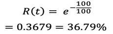
So, if you have a product with an MTBF of 100 hours, you only have a 36.79% chance that it actually functions for 100 hours!
There are a few variations of MTBF you may encounter. They are mean time between system aborts (MTBSA), mean time between critical failures (MTBCF) and mean time between unscheduled removal (MTBUR). You’ll most likely see these variations when differentiating between critical and non-critical failures.
MTBF Calculation
MTBF is calculated by taking the total time an asset is running (uptime) and dividing it by the number of breakdowns that happened over that same period of time.
MTBF = Total uptime / # of Breakdowns
Broken down, the MTBF calculation might look like this:
- Find the total uptime: Imagine you have a warehouse full of widgets, and 40 of them were tested for 400 hours each. The total hours spent testing equal 16,000 hours (40 x 400 = 16,000).
- Figure out the number of failures: Identify the number of failures over the entire number of widgets tested. For this example, consider there were 20 widget failures.
- Calculate MTBF: Now that we know testing was performed for 16,000 hours with 20 widget failures, we can calculate MTBF: 16,000 hours / 20 failures = 800 hours.
So, what does this tell us? In this example, the MTBF is not suggesting that each widget should last 800 hours. It is saying if you run a group of widgets, the average time between failures within the tested group is 800 hours. In other words, MTBF is not meant to predict the behavior of a single component; it predicts the behavior of a group of components.
It’s important to understand that when defining “time,” it may not always mean clock time; it could be the time in which the system is actually being used. For example, you may have a machine that has been run eight hours a day which might last three times as long as the exact same machine running 24 hours a day. The MTBF for both machines is the same because they both endured the same number of operating hours.
Let’s look at another example of the MTBF calculation. Let’s say you have a bottling machine designed to operate for 12 hours a day. The bottling machine breaks down after operating normally for 10 days. The MTBF in this example is 120 hours.
MTBF = (12 hours per day x 10 days) / 1 breakdown = 120 hours
The MTBF calculation requires more steps when you have longer periods of time with increasing occurrences of failures. For example, say the bottling machine that operates for 12 hours a day fails twice in 10 days. The first failure occurred 20 hours from the start time and took two hours to repair. The second failure happened 60 hours from the start time and took three hours to repair. Calculating the total uptime for the MTBF equation requires adding 20 (initial uptime period), 18 (start of first downtime period minus end of first downtime period) and 57 hours (start of second downtime period minus end of downtime period).
So, now the MTBF calculation looks like this: MTBF = (20 hours + 38 hours + 57 hours) / 2 breakdowns or 57.5 hours / 2 breakdowns = 57.5 hours.
Misunderstanding MTBF
One of the biggest misconceptions about MTBF is that it is the same thing as the number of operating hours before failure or “service life.” If you get an extremely high MTBF number (not uncommon), you might think there’s no way the system can operate this long without a failure. The reason for high MTBF numbers is because they are mostly based on the asset’s rate of failure when that asset is still in its “normal” or “useful” life, assuming it will fail at that rate forever. It’s for this reason there should be no correlation between service life and MTBF. You can have a piece of equipment with a very high MTBF but a low expected service life.
The following is a good example of MTBF misconception. Let’s say you have 500,000 25-year-olds in a sample population. Over the span of one year, data is collected on failures (deaths) for this population. The population’s operational life is 500,000 x 1 year = 500,000 people years. Over the course of the year, 625 people failed (died). This brings the failure rate to 625 failures / 500,000 people years = 0.125% / year. So, our MTBF is 1 / 0.00125 = 800 years.
This shows us that, even though 25-year-old humans have high MTBF values, their life expectancy (service rate) is a lot shorter and doesn’t correlate.
Humans, like machines, don’t exhibit a constant failure rate. As humans age, more failures occur (our bodies wear out). Since this is the case, the only way to calculate MTBF so it correlates with service life would be to wait for the whole population of 25-year-olds to reach the end of their life; then the average lifespans can be calculated. This puts that number at around 75-80 years.
So, is the MTBF for 25-year-olds 80 or 800? Torell and Avelar explain that it’s all about assumptions. In this case, the MTBF of 80 years more accurately reflects the life of the product (humans). When it comes to things like tracking products from machinery, you have many more variables, the biggest of which is time.
How to Improve MTBF
The impacts of machine failure can be significant. It leads to lost production and increased time spent on maintenance. Getting to the root cause of failures is the best way to find, mitigate or even prevent future occurrences, all while increasing your MTBF in the process. There are a few ways you can increase MTBF.
- Improve preventive maintenance processes: A well-thought-out preventive maintenance plan can greatly improve your MTBF. Anytime you can be proactive instead of reactive when it comes to maintenance, it gives you a chance to stop failures before they happen. A poorly executed preventive maintenance plan can actually have the opposite effect on MTBF. Poor training, a lack of or poorly designed manuals and checklists can all lead to quick breakdowns.
- Conduct a root cause analysis: Figuring out why something failed gives you the key to prevent that failure from happening in the future or at least from happening as often. Like preventive maintenance, root cause analysis can indirectly increase MTBF by coming up with a long-term solution. For example, if you notice a part fails fairly frequently, you may look to see if you can replace it with a higher quality part.
- Establish condition-based maintenance: If you have the ability to put into place an early warning system to detect equipment issues before they lead to failure, you can potentially increase MTBF and reduce downtime. While it’s not always easy to establish a condition-based maintenance plan, you can start by implementing a total productive maintenance plan.
Potential Issues with MTBF
It’s important to know the potential issues that could arise from an MTBF calculation when using it for reliability analysis. MTBF can differ depending on how you define certain things like “failure” and “operation time” as well as whether you measure individual pieces of equipment or a whole process.
- MTBF assumes a constant failure rate: Part of your MTBF equation is coming up with the number of failures. The issue with this shows up when there are things out of your control that result in failures, such as storms causing a power outage, short circuits due to flooding, etc. These are sometimes referred to as “acts of God” and can leave the definition of failure open to interpretation. Is a failure only a breakdown? Is a failure any time production stops no matter the cause? Should you include every type of failure when calculating MTBF, giving you a lower MTBF value? Or should you leave out certain categories of stoppages, resulting in a higher MTBF value? Be sure you know which failures are included when calculating MTBF and why those failures were chosen.
- Differing definitions of operating time: When do you consider an asset in your plant to be operating? Given the notion that parts or components are degraded by the stress they endure during operation, the greater the stress, the greater the impact of the part’s operating life. A great example of this is a car stopped at a red light. When sitting at a red light, the car’s gearbox and drivetrain are not being used, so the engine is running under the least amount of stress and suffering little wear and tear. If you were to calculate the MTBF of the idling car, would you include its idle times stopped at red lights or just the times it’s accelerating and operating at high rates of speed?
Along those same lines, should you consider operating time for your equipment as any time the equipment is turned on or only when it’s operating under normal workloads? If you choose to use the former for your MTBF calculation, your MTBF value would be higher, but that value wouldn’t be representative of machinery continually running under normal workloads and hardly ever idling. That’s why it’s important to define operating time for all assets you intend to use with MTBF.
- Choosing the equipment to monitor (bad actors): You should also determine whether you want to measure the entire process or the individual pieces of equipment within that process. One thing to note here is that an entire process suffers any time one critical asset fails. These critical assets are referred to as “bad actors” and should be flagged as causing a loss in MTBF.
Those who choose to measure an entire process for an MTBF calculation often find they can’t achieve a high MTBF value due to “bad actors.” It’s recommended to test each piece of equipment to eliminate this issue.
If you consider these potential issues ahead of time, MTBF can still be a useful tool when evaluating the reliability of your assets.