
Introduction
When solving computational problems, algorithm design is an important factor to consider because sometimes the problem requires finding the best solution from among multiple alternatives, optimizing the solution, or making decisions. Greedy algorithms and dynamic programming are two popular methods for solving such problems. Both techniques are efficient problem solving approaches, but their goals are different and yield different solutions for different problem structures. A greedy algorithm always chooses the choice that is most beneficial at the moment, but hopes that the choices will turn out to be optimal overall.
Dynamic programming, on the other hand, divides a problem into smaller manageable parts, systematically solves them, and then stores the solutions to the subproblems so they can be reused when solving other problems. Some of the concepts are explained in the context of understanding why dynamic programming is useful for specific optimization problems such as overlapping subproblems. Both techniques have applications such as scheduling tasks, finding shortest paths, allocating resources and solving the knapsack problem. Recognizing the differences enables programmers to choose the best possible solution to program efficiently, reliably, and with scalability in mind.
Greedy Algorithms
A greedy algorithm is a method of designing an algorithm that chooses optimal local solutions in order to reach the optimal global solution, but without taking into account all possible combinations of subsequent choices. It does not look at the problem as a whole, but rather chooses an option that seems most likely to help in the here and now, and takes subsequent decisions to develop the solution. This is known as “local optimization can yield a global optimum” and takes the view that having a sequence of locally superior decisions may sometimes lead to a globally optimal decision.
One type of problem in which a greedy algorithm is particularly useful is one that possesses the greedy-choice property; that is, a local optimal choice could yield an optimal overall solution. A typical instance is activity selection: the goal is to select as many mutually incompatible activities as possible. The algorithm repeatedly picks up the earliest activity to complete, leaving more time available for later activities. Unfortunately, greedy strategies are not universally applicable for optimization problems – the best choice for the short-term may be worse for the long-term.
Dynamic Programming
Dynamic programming is an algorithm design method used to solve complex problems by breaking them down into smaller subproblems, solving the subproblems and then building up an optimal solution from the subproblems. The key idea behind is to not compute the same subproblem more than once; store the results of subproblems already calculated in order to use them later. This is especially helpful if there is overlap in the subproblems and optimal substructure. The overlapping subproblems are instances in which different portions of the problem call for a solution to the same subproblem.
Optimal substructure is a characteristic of problems for which optimal solutions can be built from optimal solutions to subproblems. There are two main ways to implement dynamic programming: memoization and tabulation.Usually, a dynamic programming solution is implemented using either of two approaches: memoization and tabulation. Memoization is top-down and calculates values when they are required and stores them, and tabulation is bottom-up and works on smaller problems first and then gradually works up to the bigger problem. They are helpful in problems like the 0-1 Knapsack problem, calculating the Fibonacci numbers and some shortest-path problems.
Greedy Algorithms vs Dynamic Programming: 10 Key Differences
Greedy algorithms and dynamic programming are both applied to problems where decisions need to be made which lead to an optimization; they differ in how they make decisions, how they handle information, how they build solutions. It becomes easier to determine which technique is appropriate for a given computational problem when these differences are known. Below are 10 main differences between a greedy algorithm and a dynamic programming algorithm.
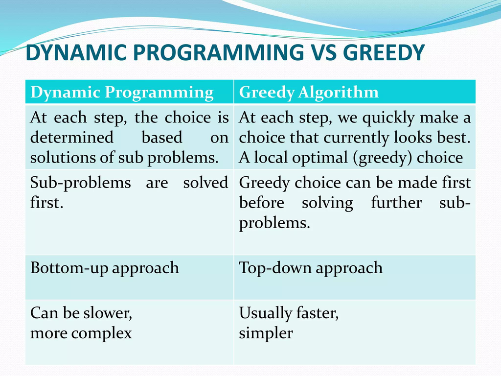
- Decision-Making Approach
The main distinction between the greedy algorithm and the dynamic programming approach is the way they decide when solving a problem. A greedy algorithm takes the best choice that is available at the moment and makes a decision. Rarely revisits past decisions even if additional information comes to light about the possibility of doing something different that would result in a better outcome. This makes the technique easy and efficient for problems in which local decisions can ensure global optimality.
Instead, dynamic programming is more systematic, it looks at how the smaller subproblems might relate to each other and evaluates possible options before choosing the best one. Instead of simply choosing an option that it likes, it will consider other options based on previously calculated values and recurrence relations. For instance, if a resource is the cheapest resource at each step it is picked, a greedy algorithm is used, but if a few combinations of resources are compared to find the one with the lowest total cost, a dynamic programming algorithm is used.
- Optimality of the Final Solution
Another significant distinction has to do with whether an algorithm will provide an optimum solution. An algorithm that has a greedy choice does not necessarily produce a globally optimal solution when it is used to solve an optimization problem. Their success is defined by whether or not the problem has the greedy choice property. If this property holds, and the algorithm has a valid greedy strategy, the approach can generate an optimal solution. But in the absence of the property, locally good choices can result in an overall bad choice. Optimisation problems that possess optimal substructure are usually better suited to dynamic programming, which will systematically evaluate the different alternatives that are relevant and add together the optimal solutions to the subproblems. For instance, a greedy algorithm can be used to find an optimum solution for the fractional knapsack problem: given a set of n items, with value v1, v2, …, vn and weights w1, w2, …, wn, respectively, where n is a positive integer, find the optimal strategy for selecting a subset of the items whose sum of values is as large as feasible for the weight constraints. The same approach is not guaranteed to give an optimal solution to the 0/1 knapsack problem, in which items can only be taken or left out. The 0/1 version of the problem can be solved using dynamic programming by taking into account various combinations of items to be selected and the capacity available.
- Handling of Subproblems
A difference between greedy algorithms and dynamic programming also lies in the way they deal with smaller parts of a problem. Generally, a greedy algorithm makes a decision based on the current state of the problem, and then proceeds without a systematic calculation of the solution to each of the important subproblems. It operates on the premise of choosing the most suitable immediate choice, and skips over combinations. Dynamic programming, however, will intentionally solve problems in a divide-and-conquer fashion, and then combine the solutions of the subproblems to get the overall solution.
If a subproblem occurs multiple times, the answer to the subproblem is computed and stored and then reused. For certain problems, such as optimization, dynamic programming is particularly useful when there are several decisions that rely on similar intermediate calculations. For example, computing the Fibonacci numbers recursively is a very simple algorithm which requires computing previous numbers several times. A way to improve this is to use dynamic programming, which stores the values of the Fibonacci numbers that have already been calculated, so that each Fibonacci number is only computed once.
- Memory Usage
Another big difference between the two is the amount of memory that is used. Greedy algorithms typically don’t need much extra memory as they only need to store the information they need to make the next decision, and the information they need to keep track of the current solution. This could be a sorted list, some variables, or a priority queue, depending on the problem. A dynamic programming solution may need more space as it will store intermediate solutions in arrays, tables, dictionaries or other data structures.
These stored values are useful for ensuring that calculations are not repeated and can efficiently be compared to different paths to the solution. For instance, the 0/1 knapsack problem is often solved using a two dimensional array to store the maximum value obtained for different sets of items and capacities. This extra memory can be used to get the correct optimisation, but it can be costly if there are lots of states in the problem. So, sometimes, programmers employ space optimization methods to minimize the amount of space used without altering the correctness of the solution.
- Time Complexity
Both greedy algorithms and dynamic programming have certain general approaches to computational problems but their time complexity depends on the problem under consideration. Greedy algorithms may be extremely efficient since they do not necessarily examine all the possibilities; they typically make a choice at a time. Some need to sort the options before feeding them into it which makes them have a time complexity of O(n\log n); some can handle them in linear time if the input is sorted in the right way.
Dynamic programming tends to make more calculations since it will calculate various states and how they are connected to each other. The time complexity of it is dependent on the number of states and the work per state. For instance, a simple solution based on dynamic programming for the 0/1 knapsack problem is of time complexity (O(nW)) where (n) is the number of items and (W) is the size of the knapsack. This is sometimes referred to as pseudo-polynomial time, since it is dependent on the numerical capacity, rather than just the number of input elements.
- Implementation Complexity
The algorithms that use greedy strategy are usually easier to implement since their decisions tend to be easy. A programmer determines the best choice for a selection criterion, arranges the alternatives if needed, and chooses the best one at the moment until the problem is completed. But this simplicity can make it easier to understand, test, and maintain greedy solutions. Dynamic programming is usually more of a planning phase since the programmer must identify the subproblems that are relevant, write the recurrence relation, decide the order in which to solve the subproblems, and choose how to store intermediate results.
Any errors during these stages may lead to wrong solutions or suboptimal implementations. Since each activity has a start and finish time, for instance, a greedy activity-selection algorithm would involve sorting the activities by finishing time and choosing the compatible activities. To find out whether adding an activity adds value to a weighted interval scheduling problem via a dynamic programming solution, extra calculations are required. This added complexity pays off if combinations can be evaluated incorrectly with a simple greedy strategy, as in the problem.
- Treatment of Previous Decisions
The principles of treating previous decisions are addressed through the following:
In a greedy algorithm, the decisions made at the start of the algorithm are not reconsidered later. After this, the algorithm is started from the selected option and new options are randomly selected depending on the information available. This is a good method to use when the preceding solutions are known to be appropriate as the solution progresses. But it can be difficult when a seemingly good choice ends up being bad. Dynamic programming deals with decision-making in a different way, by remembering the information about the various alternatives in its stored states. It doesn’t make a permanent, binding decision at the outset, but it reflects the result of each option and evaluates the options. Let’s take an example of a resource allocation problem that has multiple departments bidding for a fixed amount of funds. One of the “easy” options would be to spend cash on the department that looks like it will get the greatest return in the short term. One can use a dynamic programming technique to explore alternate allocation scenarios and see how they affect the total benefit, and decide which allocation yields the highest benefit. When decisions affect each other at several stages, this makes dynamic programming more appropriate.
- Suitable Problem Characteristics
The problems that exhibit the greedy-choice and optimal substructure properties are the most suitable to be solved with greedy algorithms. The properties enable an algorithm to make a locally optimal decision, yet has the potential to achieve a globally optimal result. For example, when building a minimum spanning tree, solving some scheduling problems, or optimizing the fractional knapsack. Dynamic programming is an efficient method for solving problems that can be divided into independent subproblems and that share overlapping subproblems. Accumulations of identical calculations may occur or when several decisions are to be compared, to determine which is most advantageous. Some examples are the 0/1 knapsack problem, the matrix chain multiplication problem, and the longest common subsequence problem. Both methods can be used for problems with optimal substructure, but merely the fact that it has optimal substructure does not make it obvious that a greedy solution will work. A programmer should also determine that the greedy-choice property is true before using a greedy algorithm and ensuring that an optimum solution is obtained.
- Performance on Large Problems
The efficiency of both methods is dependent on the structure and size of the problem, as well as the resources used for implementing the algorithm. The appeal of a greedy algorithm is that it avoids many calculations and additional memory requirements, particularly when the data set is large. For instance, a large number of activities can be processed efficiently by a suitable greedy scheduling algorithm after arranging the activities in order of finishing times. There is the possibility of using more computational resources since dynamic programming will store and process a lot of intermediate states. This can become difficult if there are many states and/or the table dimensions get large. But dynamic programming is still very efficient in many ways when compared to “brute force” methods that check all the possible solutions. It can save a tremendous amount of redundant calculations due to its use of previously computed values. Memoization, tabulation, state compression and space optimisation can be used to further enhance the performance. Hence, it is important to consider the complexity of the problem and available computational resources to decide between the two approaches.
- Flexibility and Reliability
The difference between greedy algorithms and dynamic programming is that greedy algorithms are not always reliable when problems have complicated decision relationships while dynamic programming is always reliable in this situation. Greedy algorithms work well if the problem can be structured to follow a certain local decision rule, but can be inappropriate if subsequent decisions can have significant impact on the quality of previous decisions. The correctness of their procedures is frequently dependent on demonstrating that each greedy choice is safe. For many optimization problems, the flexibility of dynamic programming allows different states to be represented, different possible decisions can be compared and previously calculated results can be combined.
It is applicable to problems that involve making a choice which will affect future options. But dynamic programming doesn’t always solve the most optimal optimization problem. There are some problems that can have too many states, which would make the approach too costly or impractical. The best approach is to analyse the math properties of the problem, what guarantees are needed, and to select an algorithm with the appropriate structure.
Real-life Applications of Greedy Algorithms and Dynamic Programming
It is helpful to know the differences between these techniques but helpful examples illustrate their applications. Different algorithms are selected for different problem variants as seen in scheduling, shortest-path problems, resource allocation and knapsack optimization.

- Scheduling Problems
Scheduling problems are problems of arranging activities, jobs or tasks satisfying specific constraints. One is the activity selection problem: an individual has a certain number of activities that start and end at various points in time, but can only be involved in one activity at a time. The goal is to choose the most activities possible that do not conflict. The solution to this is a greedy algorithm that sorts the list of activities by their end times and chooses, in sequence, the next activity that fits, which has the earliest end time.
This approach is best because the activity that is scheduled for the earliest completion time will have the most time left for other activities to complete. But when each activity pays a different amount or is more important than another activity, scheduling becomes more complicated. The goal of weighted interval scheduling is to select the most valuable set of activities, not just the largest set of activities. This version is best suited for dynamic programming, which considers the value of performing an activity versus not performing it, and considers previous compatible activities.
- Shortest-Path Problems
Shortest-path problems are used to find the shortest path (lowest cost) between two locations or nodes in a graph. Such a problem is seen in transportation systems, communication networks, navigation applications and logistics platforms. Dijkstra’s algorithm is a well-known greedy algorithm that finds the shortest path from a given vertex in a graph where all the edge weights are non-negative. It keeps marking the vertex which has the smallest tentative distance that it hasn’t visited and updates the tentative distances of the adjacent vertices. This strategy ensures the proper shortest distances under the non-negative edge-weight constraint.
In general, Dijkstra’s algorithm does not work correctly on graphs which have edges with negative weight. Other algorithms, like Bellman-Ford, are able to cope with negative weights on the edges and with finding reachable negative-weight cycles. Bellman-Ford is a repeated version of relaxing the edges of the graph and can be understood by dynamic programming since it constructs shortest-path information over increasing numbers of edges. This example supports the notion that the important thing when picking an algorithm is to understand the constraints of the problem.
- Resource Allocation Problems
Resource allocation is the process of allocating scarce resources among competing activities, departments or projects to maximise the value. Resources could be financial, computing, people, storage, materials, etc. A greedy strategy may be helpful if each allocation can be judged individually, and if there is a local optimum choice that is always helpful in achieving the overall goal. When the structure of the problem is such that an efficient measure has been well defined, an organization may compute this measure for various projects and choose those with the lowest value. In the real world, however, interacting constraints, varying project values and limited capacities occur in real world resource allocation. In such cases, dynamic programming can be used to compare the various sets of allocations and select the one that yields the greatest overall benefit. States can be used to represent a budget allocation problem, where each state represents some amount of money available and which projects have been considered. The algorithm then finds the optimum solution for each state, thus allowing the determination of an effective allocation of the scarce resources.
- The Knapsack Problem
The knapsack problem is one of the clearest examples of the differences between greedy algorithms and dynamic programming. It involves selecting items with different weights and values while ensuring that their combined weight does not exceed a specified capacity. In the fractional knapsack problem, items can be divided into smaller portions, allowing a greedy algorithm to select items according to their value-to-weight ratios. By prioritizing the items that provide the greatest value per unit of weight, the algorithm produces an optimal result.
However, the 0/1 knapsack problem imposes a different restriction: each item must either be selected completely or left behind. A greedy approach based on value-to-weight ratios may fail because selecting an attractive item can prevent a better combination of smaller items from fitting into the available capacity. Dynamic programming solves this version by evaluating whether each item should be included or excluded while tracking the remaining capacity. It can therefore identify the optimal combination of items for the given constraints.
Advantages of Greedy Algorithms
Greedy algorithms offer several advantages that make them useful in practical software development and computational problem-solving. Their most significant benefit is simplicity because they usually follow a straightforward decision-making process that is easy to implement and understand. They can also be computationally efficient, particularly when the problem allows a solution to be constructed through a sequence of locally optimal decisions. Since they generally require limited additional memory, they can be suitable for applications involving large datasets or systems with restricted resources.
Another advantage is that many greedy algorithms can produce solutions without exploring every possible combination of choices. This makes them valuable in areas such as network design, scheduling, graph processing, and optimization. However, these advantages depend on selecting an appropriate greedy strategy. A simple implementation does not necessarily mean that the result is correct or optimal. Developers must establish the mathematical properties of the problem before deciding that a greedy algorithm is appropriate.
Advantages of Dynamic Programming
Dynamic programming provides important advantages when solving optimization problems that require comparing several possible decisions. Its main strength is its ability to avoid repeated calculations by storing intermediate results and reusing them whenever necessary. This can significantly improve performance compared with ordinary recursive solutions that repeatedly solve identical subproblems. Dynamic programming is also effective when the objective is to guarantee an optimal solution and the problem has the necessary mathematical properties.
By systematically examining possible states and combining their solutions, it can handle situations where an immediate local choice might produce a poor overall outcome. Its applications extend to financial planning, scheduling, resource allocation, text processing, computational biology, and artificial intelligence. Furthermore, dynamic programming can provide a clear mathematical framework for understanding complicated optimization challenges. Despite these strengths, its implementation can require substantial memory, careful state design, and more development time than a simpler greedy solution.
Limitations of Greedy Algorithms and Dynamic Programming
Despite their usefulness, neither technique is suitable for every computational problem. Greedy algorithms have the limitation of depending heavily on the problem’s structure. When the greedy-choice property does not hold, selecting the best immediate option may prevent the algorithm from finding the globally optimal solution. Another challenge is that proving the correctness of a greedy strategy can be difficult, particularly when the problem involves several interacting constraints. Dynamic programming also has limitations, especially when the number of possible states becomes extremely large.
A problem with several dimensions, large input values, or numerous decision variables may require significant processing time and memory. Designing the correct recurrence relationship can also be challenging, and an incorrectly defined state may lead to an incomplete or inefficient solution. In some cases, alternative techniques such as divide and conquer, backtracking, approximation algorithms, or heuristic methods may be more appropriate. Developers should therefore evaluate the complexity, constraints, and expected output of a problem before selecting an approach.
How to Choose Between Greedy Algorithms and Dynamic Programming
Choosing between greedy algorithms and dynamic programming begins with understanding the structure of the optimization problem. Developers should first identify the objective, constraints, and decisions required to produce a valid solution. The next step is to determine whether a locally optimal decision can always be part of a globally optimal solution. If this can be established through the greedy-choice property, a greedy algorithm may provide an efficient and straightforward solution. If the problem contains overlapping subproblems and requires comparing different combinations of decisions, dynamic programming may be more appropriate.
Programmers should also consider the number of possible states, available memory, input size, and expected execution time. Testing different approaches against carefully selected examples can reveal situations where a seemingly reasonable greedy strategy fails. For more complicated problems, mathematical reasoning and correctness proofs are important before implementation. Ultimately, the best technique is not necessarily the one with the shortest code but the one that produces correct results efficiently under the problem’s actual constraints.
Real-World Applications of Both Techniques
Greedy algorithms and dynamic programming support many applications in modern computing and technology. Greedy algorithms are commonly used in network optimization, minimum spanning tree construction, data compression, scheduling, and certain routing problems. For example, Kruskal’s and Prim’s algorithms use greedy strategies to construct minimum spanning trees, which help connect network components at minimum total edge cost. Huffman coding also uses a greedy approach to construct efficient prefix codes for data compression. Dynamic programming is widely applied in artificial intelligence, natural language processing, financial optimization, computational biology, and decision-support systems.
It can help compare sequences of characters, optimize resource distribution, and calculate solutions to complex decision problems. In computational biology, for instance, dynamic programming is used in sequence alignment to identify similarities between DNA or protein sequences. In business applications, it can support planning decisions involving limited budgets, production capacity, and competing priorities. These examples demonstrate that both techniques remain important because different computational challenges require different methods of optimization.
Conclusion
Greedy algorithms and dynamic programming are two important algorithm design techniques that help programmers solve optimization problems, but they approach decision-making in fundamentally different ways. Greedy algorithms select the best available option at each stage and are particularly effective when local decisions can be proven to produce a globally optimal result. Their simplicity, low memory requirements, and potential for fast execution make them valuable for problems such as activity selection, minimum spanning tree construction, and fractional knapsack optimization.
Dynamic programming takes a more comprehensive approach by dividing problems into smaller subproblems, storing intermediate results, and comparing possible decisions to construct an optimal solution. This makes it suitable for challenges such as the 0/1 knapsack problem, weighted interval scheduling, and sequence alignment. Neither approach is universally superior, and the correct choice depends on the mathematical properties, constraints, and computational requirements of the problem. By understanding their differences and recognizing when each technique is appropriate, developers can design more efficient algorithms and build reliable solutions to complex computational challenges.